Estimating the Gaussian Distribution
The math of estimating the parameters of a Gaussian using MLE as well as Bayesian inference, with some intuition regarding the effects of sample size and prior selection.
← The Gaussian DistributionLinear Regression →
In the previous post we saw the definition of the Gaussian distribution and some of its most useful properties. Having defined this distribution, our next point of interest will be to estimate the mean and covariance of a Gaussian distribution given some datapoints. This will be our main focus in this post.
While Bayesian statistics is our main interest in this thread of posts, many times it’s easier to go over the frequentist version first, since it’s less mathematically involved. Once we understand the ML solution, we will move on to the Bayesian treatment. Many times, this process reveals how the Bayesian and frequentist views are related to each other.
The parameters of a Gaussian distribution are $\mu$ and $\Sigma$, so \(\theta=\left\{ \mu,\Sigma\right\}\) . In the frequentist case we will estimate both, however the Bayesian treatment of $\Sigma$ is a bit more complex and doesn’t teach much, so we will ignore it for now.
ML Estimates
The log-likelihood of a data set \(\mathcal{D}=\left\{ x_{i}\right\} _{i=1}^{N}\) sampled from a Gaussian distribution is:
\[\begin{equation} \begin{split}\log p\left(\mathcal{D}|\mu,\Sigma\right) & =\sum_{i}\log\mathcal{N}\left(x_{i}\,|\,\mu,\Sigma\right)\\ & =\sum_{i}\log\left[\frac{1}{\sqrt{\left(2\pi\right)^{d}\left|\Sigma\right|}}\exp\left\{ -\frac{1}{2}\left(x_{i}-\mu\right)^{T}\Sigma^{-1}\left(x_{i}-\mu\right)\right\} \right]\\ & =\sum_{i}\left[-\frac{d}{2}\log2\pi-\frac{1}{2}\log\left|\Sigma\right|-\frac{1}{2}\left(x_{i}-\mu\right)^{T}\Sigma^{-1}\left(x_{i}-\mu\right)\right]\\ & =-\frac{Nd}{2}\log2\pi-\frac{N}{2}\log\left|\Sigma\right|-\frac{1}{2}\sum_{i}\left(x_{i}-\mu\right)^{T}\Sigma^{-1}\left(x_{i}-\mu\right) \end{split} \end{equation}\]Before we begin the process of finding the ML estimators
Now, recall that $\left(x-\mu\right)^{T}\Sigma^{-1}\left(x-\mu\right)$ is also a scalar, so we can use the above identity to rewrite it as:
\[\begin{align} \ell\left(\mathcal{D}|\mu,\Sigma\right) & =-\frac{Nd}{2}\log2\pi-\frac{N}{2}\log\left|\Sigma\right|-\frac{1}{2}\sum_{i}\text{trace}\left[\Sigma^{-1}\left(x_{i}-\mu\right)\left(x_{i}-\mu\right)^{T}\right]\nonumber \\ & =-\frac{Nd}{2}\log2\pi-\frac{N}{2}\log\left|\Sigma\right|-\frac{1}{2}\text{trace}\left[\Sigma^{-1}\sum_{i}\left(x_{i}-\mu\right)\left(x_{i}-\mu\right)^{T}\right] \end{align}\]Finally, if we define $S\stackrel{\Delta}{=}\frac{1}{N}\sum_{i}\left(x_{i}-\mu\right)\left(x_{i}-\mu\right)^{T}$ (which is almost the empirical covariance), we get a shorter form for the log-likelihood (which is sometimes used in the literature):
\[\begin{equation} \ell\left(\mathcal{D}|\mu,\Sigma\right)=-\frac{N}{2}\left(d\log2\pi+\log\left|\Sigma\right|+\text{trace}\left[\Sigma^{-1}S\right]\right) \end{equation}\]MLE for $\mu$
We begin by finding the mean that maximizes the log-likelihood, by differentiating the log-likelihood:
\[\begin{align} \frac{\partial\ell}{\partial\mu} & =-\frac{1}{2}\sum_{i}\frac{\partial}{\partial\mu}\left(x_{i}-\mu\right)^{T}\Sigma^{-1}\left(x_{i}-\mu\right)\\ & =-\frac{1}{2}\sum_{i}2\Sigma^{-1}\left(x_{i}-\mu\right)\\ & =-\Sigma^{-1}\sum_{i}\left(x_{i}-\mu\right)\stackrel{!}{=}0 \end{align}\]By equating to 0 we can find the maxima:
\[\begin{equation} \hat{\mu}_{\text{ML}}=\frac{1}{N}\sum_{i}x_{i} \end{equation}\]Here we write $\hat{\mu}_{\text{ML}}$ to show that it is the maximum likelihood estimator for the data set. Notice that, unsurprisingly, the ML estimator for the mean of the Gaussian is the empirical mean of the data.
MLE for $\Sigma$
Using the following definition of the derivatives (which are a bit harder to get directly on your own):
\[\begin{equation} \frac{\partial}{\partial\Sigma}\log\left|\Sigma\right|=\frac{1}{\left|\Sigma\right|}\frac{\partial}{\partial\Sigma}\left|\Sigma\right|=\frac{1}{\left|\Sigma\right|}\left|\Sigma\right|\Sigma^{-1}=\Sigma^{-1} \end{equation}\]and:
\[\begin{equation} \frac{\partial}{\partial\Sigma}\text{trace}\left[\Sigma^{-1}S\right]=-\Sigma^{-1}S\Sigma^{-1} \end{equation}\]we can find the MLE for $\Sigma$. The full derivative of the log-likelihood by $\Sigma$ is:
\[\begin{align} \frac{\partial\ell}{\partial\Sigma} & =-\left(\Sigma^{-1}-\Sigma^{-1}S\Sigma^{-1}\right)\stackrel{!}{=}0\nonumber \\ \Rightarrow & \Sigma^{-1}=\Sigma^{-1}S\Sigma^{-1}\nonumber \\ \Rightarrow & I=\Sigma^{-1}S\nonumber \\ \Rightarrow & \Sigma=S\nonumber \\ \Rightarrow & \hat{\Sigma}_{\text{ML}}=\frac{1}{N}\sum_{i}\left(x_{i}-\mu\right)\left(x_{i}-\mu\right)^{T} \end{align}\]Because $\hat{\mu}_{\text{ML}}$ is not dependent on $\hat{\Sigma}_{\text{ML}}$, we can first find the MLE for $\mu$ and then for $\Sigma$ , so that:
\[\begin{equation} \hat{\Sigma}_{\text{ML}}=\frac{1}{N}\sum_{i}\left(x_{i}-\hat{\mu}_{\text{ML}}\right)\left(x_{i}-\hat{\mu}_{\text{ML}}\right)^{T} \end{equation}\]Putting the two equations together, the ML estimators for the parameters of a Gaussian distribution are: \(\begin{equation} \begin{split}\hat{\mu}_{\text{ML}} & =\frac{1}{N}\sum_{i}x_{i}\\ \hat{\Sigma}_{\text{ML}} & =\frac{1}{N}\sum_{i}\left(x_{i}-\hat{\mu}_{\text{ML}}\right)\left(x_{i}-\hat{\mu}_{\text{ML}}\right)^{T} \end{split} \end{equation}\)
1D Bayesian Inference
Recall that in the Bayesian treatment, we assume that the parameters are distributed in some manner. We begin by considering the 1D case for Gaussian distributions
For now, we will assume that we know the variance $\sigma^{2}$ . We will assume a Gaussian prior over $\mu$ (if we want we can assume different priors as well, but let’s stick with Gaussian priors for now):
\[\begin{equation} p\left(\mu\right)=\mathcal{N}\left(\mu_{0},\sigma_{0}^{2}\right) \end{equation}\]Given a data set $\mathcal{D}=\left{ x_{i}\right} _{i=1}^{N}$ , the likelihood is:
\[\begin{align} p\left(\mathcal{D}|\mu\right) & =\prod_{i=1}^{N}p\left(x_{i}|\mu\right)=\prod_{i=1}^{N}\mathcal{N}\left(x_{i}\,|\,\mu,\sigma^{2}\right)\\ & \propto\exp\left[-\frac{1}{2\sigma^{2}}\sum_{i=1}^{N}\left(x_{i}-\mu\right)^{2}\right] \end{align}\]The posterior probability for $\mu$ will then be:
\[\begin{align}\label{eq:post} p\left(\mu|\mathcal{D}\right) & =\frac{p\left(\mathcal{D}|\mu\right)p\left(\mu\right)}{p\left(\mathcal{D}\right)}\\ & \propto p\left(\mathcal{D}|\mu\right)p\left(\mu\right) \end{align}\]Recall that the term $p\left(\mathcal{D}\right)$ is constant and only serves as a normalization, so for now we can ignore it.
Derivation of the posterior
Let’s look at the product in equation \eqref{eq:post} more closely:
\[\begin{align} p\left(\mathcal{D}|\mu\right)p\left(\mu\right) & \propto\exp\left[-\frac{1}{2\sigma^{2}}\sum_{i=1}^{N}\left(x_{i}-\mu\right)^{2}\right]\exp\left[-\frac{\left(\mu-\mu_{0}\right)^{2}}{2\sigma_{0}^{2}}\right]\\ & =\exp\left[-\frac{1}{2}\left(\frac{1}{\sigma^{2}}\sum_{i=1}^{N}\left(x_{i}-\mu\right)^{2}+\frac{1}{\sigma_{0}^{2}}\left(\mu-\mu_{0}\right)^{2}\right)\right] \end{align}\]Notice that the term in the exponent is still quadratic in $\mu$ . This means, of course, that this whole term is still a Gaussian distribution. Let’s use the derivative trick from the previous post in order to find the distribution of $\mu$ exactly. Define:
\[\begin{equation} \Delta\stackrel{\Delta}{=}\frac{1}{2}\left(\frac{1}{\sigma^{2}}\sum_{i=1}^{N}\left(x_{i}-\mu\right)^{2}+\frac{1}{\sigma_{0}^{2}}\left(\mu-\mu_{0}\right)^{2}\right) \end{equation}\]Recall, we can now differentiate $\Delta$ with respect to $\mu$ in order to find the mean and covariance of the posterior distribution:
\[\begin{align} \frac{\partial\Delta}{\partial\mu} & =\frac{1}{2}\left(\frac{1}{\sigma^{2}}\sum_{i}\frac{\partial}{\partial\mu}\left(x_{i}-\mu\right)^{2}+\frac{1}{\sigma_{0}^{2}}\frac{\partial}{\partial\mu}\left(\mu-\mu_{0}\right)^{2}\right)\nonumber \\ & =\frac{1}{\sigma^{2}}\sum_{i}\left(\mu-x_{i}\right)+\frac{1}{\sigma_{0}^{2}}\left(\mu-\mu_{0}\right)\nonumber \\ & =\frac{1}{\sigma^{2}}\left(N\mu-\sum_{i}x_{i}\right)+\frac{1}{\sigma_{0}^{2}}\left(\mu-\mu_{0}\right)\nonumber \\ & =\frac{N}{\sigma^{2}}\left(\mu-\mu_{ML}\right)+\frac{1}{\sigma_{0}^{2}}\left(\mu-\mu_{0}\right)\nonumber \\ & =\left(\frac{N}{\sigma^{2}}+\frac{1}{\sigma_{0}^{2}}\right)\left(\mu-\left(\frac{N}{\sigma^{2}}+\frac{1}{\sigma_{0}^{2}}\right)^{-1}\left(\frac{N}{\sigma^{2}}\mu_{\text{ML}}+\frac{1}{\sigma_{0}^{2}}\mu_{0}\right)\right) \end{align}\]where $\mu_{\text{ML}}=\frac{1}{N}\sum_{i}x_{i}$ is the ML estimate for $\mu$ , as we showed in section for the MLE of the mean .
Defining: \(\begin{equation} \frac{N}{\sigma^{2}}+\frac{1}{\sigma_{0}^{2}}\stackrel{\Delta}{=}\frac{1}{\sigma_{N}^{2}} \end{equation}\) the posterior of $\mu$ is equal to:
\[\begin{equation} p\left(\mu|\mathcal{D}\right)=\mathcal{N}\left(\mu\,|\,\sigma_{N}^{2}\left(\frac{N}{\sigma^{2}}\mu_{\text{ML}}+\frac{1}{\sigma_{0}^{2}}\mu_{0}\right),\,\sigma_{N}^{2}\right) \end{equation}\]where $\sigma_{N}^{2}=\left(\frac{N}{\sigma^{2}}+\frac{1}{\sigma_{0}^{2}}\right)^{-1}=\left(\frac{N\sigma_{0}^{2}+\sigma^{2}}{\sigma_{0}^{2}\sigma^{2}}\right)^{-1}=\frac{\sigma_{0}^{2}\sigma^{2}}{N\sigma_{0}^{2}+\sigma^{2}}$ and $\mu_{\text{ML}}=\frac{1}{N}\sum_{i}x_{i}$ . If we write all of this explicitly, we will get:
\[\begin{equation} p\left(\mu|\mathcal{D}\right)=\mathcal{N}\left(\mu\,|\,\frac{\sigma_{0}^{2}\sigma^{2}}{N\sigma_{0}^{2}+\sigma^{2}}\left(\frac{N}{\sigma^{2}}\mu_{\text{ML}}+\frac{1}{\sigma_{0}^{2}}\mu_{0}\right),\,\frac{\sigma_{0}^{2}\sigma^{2}}{N\sigma_{0}^{2}+\sigma^{2}}\right) \end{equation}\]Effects of Sample Size
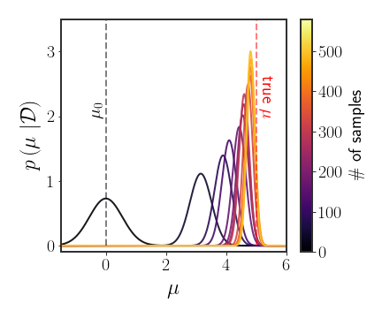
It may be a good idea to get some intuition for the posterior we found. Let’s look at the slightly simpler case of $\mu_{0}=0$ (but the analysis that follows is true for any $\mu_{0}$ ). In this case, the posterior is:
\[\begin{equation} \mathcal{N}\left(\frac{\sigma_{0}^{2}\sigma^{2}}{N\sigma_{0}^{2}+\sigma^{2}}\cdot\frac{N}{\sigma^{2}}\mu_{\text{ML}},\,\frac{\sigma_{0}^{2}\sigma^{2}}{N\sigma_{0}^{2}+\sigma^{2}}\right) \end{equation}\]Let’s see what happens when $N=0$ . If we don’t have any data, we should probably always fall back to the only thing we know; our prior. At $N=0$ , we have:
\[\begin{equation} N=0\qquad\begin{array}{c} \frac{\sigma_{0}^{2}\sigma^{2}}{N\sigma_{0}^{2}+\sigma^{2}}\cdot\frac{N}{\sigma^{2}}\mu_{\text{ML}}=0=\mu_{0}\\ \frac{\sigma_{0}^{2}\sigma^{2}}{N\sigma_{0}^{2}+\sigma^{2}}=\frac{\sigma_{0}^{2}\sigma^{2}}{\sigma^{2}}=\sigma_{0}^{2} \end{array} \end{equation}\]so the posterior (naturally) falls back to the prior. If we look at the other extreme, $N\rightarrow\infty$ , then there should be no ambiguity over the value of $\mu$ whatsoever:
\[\begin{equation} N\rightarrow\infty\qquad\begin{array}{c} \frac{\sigma_{0}^{2}\sigma^{2}}{N\sigma_{0}^{2}+\sigma^{2}}\cdot\frac{N}{\sigma^{2}}\mu_{\text{ML}}\rightarrow\frac{\sigma_{0}^{2}\sigma^{2}}{N\sigma_{0}^{2}}\cdot\frac{N}{\sigma^{2}}\mu_{\text{ML}}=\mu_{\text{ML}}\\ \frac{\sigma_{0}^{2}\sigma^{2}}{N\sigma_{0}^{2}+\sigma^{2}}\rightarrow\frac{\sigma_{0}^{2}\sigma^{2}}{N\sigma_{0}^{2}}=0 \end{array} \end{equation}\]If $N$ is somewhere in between, then the term for the mean is (as we saw before): \(\begin{equation}\label{eq:mu-N} \mu_{N}\stackrel{\Delta}{=}\left(\frac{N}{\sigma^{2}}+\frac{1}{\sigma_{0}^{2}}\right)^{-1}\left(\frac{N}{\sigma^{2}}\mu_{\text{ML}}+\frac{1}{\sigma_{0}^{2}}\mu_{0}\right) \end{equation}\) This is a weighted mean of the two values $\mu_{\text{ML}}$ and $\mu_{0}$ (you can find a demo for this behavior here). We can look at the number of samples needed in order for $\mu_{N}$ to be exactly between the ML estimate and the prior by giving equal weight to both terms:
\[\begin{equation} \frac{N}{\sigma^{2}}\stackrel{!}{=}\frac{1}{\sigma_{0}^{2}}\Rightarrow\hat{N}=\frac{\sigma^{2}}{\sigma_{0}^{2}} \end{equation}\]So, when the variance of the prior is very small, which is like saying “we are very sure that $\mu$ is close to $\mu_{0}$ “, then a lot of samples are needed in order to move $\mu_{N}$ away from the prior $\mu_{0}$ . If, on the other hand, the variance of the prior is very large, which may mean we are very unsure that $\mu_{0}$ is correct, then few points are needed in order to move the mean from the prior mean. Finally, if the sample variance ( $\sigma^{2}$ ) is very large, then we need to get a lot of data to be sure that the MLE is correct, while if it is very small, then we need very few points in order to be sure of the MLE.
Because the posterior is so dependent on the number of samples, it is sometimes written (like in equation \eqref{eq:mu-N}) as:
\[\begin{equation} p\left(\mu|\mathcal{D}\right)=\mathcal{N}\left(\mu\,|\,\mu_{N},\sigma_{N}^{2}\right) \end{equation}\]with the intention behind this notation being “this is the posterior mean after having sampled $N$ points”.
MAP and MMSE Estimates for $\mu$
The MAP estimate for $\mu$ under the prior above is given by:
\[\begin{equation} \hat{\mu}_{\text{MAP}}=\arg\max_{\mu}p\left(\mu|\mathcal{D}\right)=\arg\max_{\mu}\mathcal{N}\left(\mu\,|\,\mu_{N},\sigma_{N}^{2}\right) \end{equation}\]Of course, the Gaussian distribution only has one maxima, which is the mean of the distribution. So the MAP estimate of $\mu$ is simply the mean:
\[\begin{equation} \hat{\mu}_{\text{MAP}}=\mathbb{E}\left[p\left(\mu|\mathcal{D}\right)\right]=\mu_{N} \end{equation}\]where $\mu_{N}$ is given explicitly in equation \eqref{eq:mu-N}. Notice that (in this case) the MAP and MMSE estimates are one and the same: \(\begin{equation} \hat{\mu}_{MAP}=\mathbb{E}\left[p\left(\mu|\mathcal{D}\right)\right]=\hat{\mu}_{MMSE} \end{equation}\) The fact that the MAP and MMSE estimates are the same only happens to be true for the Gaussian distribution, in general they might be very different from each other!
Multivariate Gaussian
Now that we understood the basic premise of the Bayesian inference for $\mu$ in 1D, we can start all over again for the multivariate case. We assume, again, that: \(\begin{equation} x\sim\mathcal{N}\left(\mu,\Sigma\right) \end{equation}\) where the covariance matrix $\Sigma$ is known. We also assume a prior over $\mu$ of the form: \(\begin{equation} \mu\sim\mathcal{N}\left(\mu_{0},\Sigma_{0}\right) \end{equation}\) The likelihood for a data set $\mathcal{D}$ is: \(\begin{equation} p\left(\mathcal{D}|\mu\right)\propto\exp\left[-\frac{1}{2}\sum_{i=1}^{N}\left(x_{i}-\mu\right)^{T}\Sigma^{-1}\left(x_{i}-\mu\right)\right] \end{equation}\) and the posterior is:
\[\begin{equation} p\left(\mu|\mathcal{D}\right)\propto\exp\left[-\frac{1}{2}\sum_{i=1}^{N}\left(x_{i}-\mu\right)^{T}\Sigma^{-1}\left(x_{i}-\mu\right)\right]\exp\left[-\frac{1}{2}\left(\mu-\mu_{0}\right)^{T}\Sigma_{0}^{-1}\left(\mu-\mu_{0}\right)\right] \end{equation}\]Essentially nothing has changed from before; the term in the exponent is still quadratic in $\mu$, so we can employ our tricks once again:
\[\begin{align*} \frac{\partial}{\partial\mu}\Delta & =\Sigma^{-1}\sum_{i}\left(\mu-x_{i}\right)+\Sigma_{0}^{-1}\left(\mu-\mu_{0}\right)\\ & =N\Sigma^{-1}\left(\mu-\mu_{\text{ML}}\right)+\Sigma_{0}^{-1}\left(\mu-\mu_{0}\right)\\ & =\left(N\Sigma^{-1}+\Sigma_{0}^{-1}\right)\left[\mu-\left(N\Sigma^{-1}+\Sigma_{0}^{-1}\right)^{-1}\left(N\Sigma^{-1}\mu_{\text{ML}}+\Sigma_{0}^{-1}\mu_{0}\right)\right] \end{align*}\]where we used the same definition as before for $\mu_{\text{ML}}$ (the ML estimate for $\mu$ ). The full posterior is given by: \(\begin{equation} \mu|\mathcal{D}\sim\mathcal{N}\left(\mu_{N},\Sigma_{N}\right) \end{equation}\) where: \(\begin{align} \Sigma_{N} & =\left[N\Sigma^{-1}+\Sigma_{0}^{-1}\right]^{-1}\\ \mu_{N} & =\Sigma_{N}\left[N\Sigma^{-1}\mu_{\text{ML}}+\Sigma_{0}^{-1}\mu_{0}\right] \end{align}\)
The result is consistent with what we saw in 1D. The main difference here is that now we need to invert the matrix $N\Sigma^{-1}+\Sigma_{0}^{-1}$ in order to find $\Sigma_{N}$ and $\mu_{N}$ . The MAP/MMSE estimates for the multivariate $\mu$ are again the mean of the posterior (since this is a Gaussian distribution as well): \(\begin{equation} \hat{\mu}_{\text{MAP}}=\left[N\Sigma^{-1}+\Sigma_{0}^{-1}\right]^{-1}\left[N\Sigma^{-1}\mu_{\text{ML}}+\Sigma_{0}^{-1}\mu_{0}\right]=\hat{\mu}_{MMSE} \end{equation}\)
Choices of Priors
When theoretically analyzing Bayesian methods, they are often described in terms of “the true prior”. However, in practice we don’t actually have explicit access to “the true prior” and instead have to choose which prior to use. This is the main criticism against the Bayesian approach, because when there is not much prior knowledge researchers tend to choose arbitrary distributions as their priors.
The fact that a prior can be chosen, however, does give a lot of flexibility. If a researcher understands that their prior knowledge isn’t very good, they can assign a very “wide” prior - one that gives similar densities to most parameter settings. Choosing a wide prior then has the effect of only slightly biasing the MLE. On the flip side, if there is a lot of prior knowledge, then it only seems natural to take that knowledge into account.
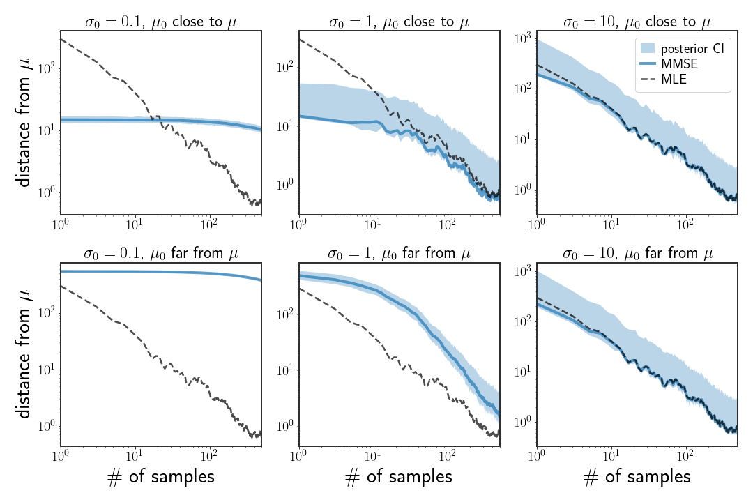
The figure above illustrates what happens when Gaussian priors of different kinds are chosen. When the variance of the prior is low, i.e. $\Sigma_{0}=I\sigma_{0}^{2}$ with small $\sigma$ (left column), then many samples are needed to change the posterior distribution. When the prior mean is well calibrated to the generating distribution but the variance is still small, this translates to a better MMSE than the ML estimate with few samples but doesn’t get better when more samples are introduced. However, when the prior mean is far from the generating distribution, then the estimate will always be quite bad if the variance is kept small. The other end of the spectrum is when $\sigma$ is large (right column), in which case it doesn’t really matter what the prior mean is since the posterior mean is more or less equal to the ML estimate.
The more interesting case is when $\mu_{0}$ is well calibrated and $\Sigma_{0}$ is moderate (middle column, top). In this setting, the MMSE gives a much better estimate than the MLE, especially in low sample-size settings - in this case, more than an order of magnitude.
All of this is to say that the choice of prior can, and sometimes should, have big effects on estimates. Choosing a well calibrated prior, something we will look into in a few posts but can be done.
Discussion
Even though the Gaussian distribution is one of the simplest distributions we can work with, it already illustrates the effects of using the Bayesian approach, which we saw in the previous section. When the prior is correctly specified, it can greatly boost performance in the low-data regime; on the other hand, when the amount of observed data increases, this posterior “merges” with the ML solution.
In the next few posts we will still be concerned with the Gaussian distribution, however we will cast the problem into that of prediction in the regression task. Basically, we will observe what we consider to be a linear transformation of a Gaussian, and we will once again attempt to recover the parameters of the Gaussian.