The Gaussian Distribution
The Gaussian distribution is hands-down the most-used distribution in machine learning. This post will go through key aspects of the normal distribution and its representations.
← Estimation and Bayes-Optimal EstimatorsEstimating the Gaussian Distribution →
The distribution that is used most often in ML (and statistics) is the Gaussian distribution, also called the normal distribution. The reason this distribution is so commonly used is because of two reasons: it is empirically observed in the wild many times and, perhaps more importantly, it is mathematically very simple to use. This post will delve into the definition and properties of the Gaussian distribution
Definition
A random variable $x$ is said to have a Gaussian distribution if it’s PDF has the following form:
\(\begin{equation} p\left(x\right)=\frac{1}{\sqrt{2\pi\sigma^{2}}}\exp\left[-\frac{1}{2\sigma^{2}}\left(x-\mu\right)^{2}\right] \end{equation}\) Notice that this distribution can be completely described by the two parameters $\mu$ and $\sigma$ - the mean and variance of the Gaussian. Because of this, we will usually write:
\(\begin{equation} x\sim\mathcal{N}\left(\mu,\sigma^{2}\right) \end{equation}\) to indicate that $x$ is a Gaussian random variable, with the two parameters $\mu$ and $\sigma$ . In the same manner, we denote the PDF by:
\[\begin{equation} p\left(x\right)=\mathcal{N}\left(x\,\mid \,\mu,\sigma^{2}\right)\qquad{\scriptstyle \left(\equiv\mathcal{N}\left(x\,;\,\mu,\sigma^{2}\right)\right)} \end{equation}\]The conditioning sign (or semi-colon) in $\mathcal{N}\left(x\,\mid \,\mu,\sigma^{2}\right)$ is to show that $x$ is the variable that we are interested in, while $\mu$ and $\sigma$ are the parameters that define the distribution (so, given a $\mu$ and a $\sigma$, we know the PDF of $x$ ).
The multivariate version for a $d$ -dimensional random vector $x\in\mathbb{R}^{d}$ is defined as:
\[\begin{equation} \mathcal{N}\left(x\,\mid \,\mu,\Sigma\right)=\frac{1}{\sqrt{\left(2\pi\right)^{d}\mid \Sigma\mid }}\exp\left[-\frac{1}{2}\left(x-\mu\right)^{T}\Sigma^{-1}\left(x-\mu\right)\right] \end{equation}\]and in this case $\mu$ is also a vector and $\Sigma$ is a symmetrical $n\times n$ matrix. The term $D_{M}\left(x\,\mid \,\mu,\Sigma\right)^{2}=\left(x-\mu\right)^{T}\Sigma^{-1}\left(x-\mu\right)$ is often called the Mahalanobis distance and is denoted with $\Delta$. The multivariate version for the Gaussian distribution is also called the multivariate normal (MVN) distribution.
Geometry of the Gaussian Distribution
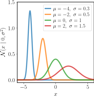
In 1D, the Gaussian distribution takes the form of the famous bell curve in figure 1 and is easy to view. However, in multiple dimensions it is not so clear what the geometry of the distribution actually looks like. We can gain insight by considering the EVD of the covariance matrix $\Sigma$ (remember, this decomposition exists since $\Sigma$ is symmetric):
\(\Sigma=UDU^{T}\) where $D$ is a diagonal matrix with the eigenvalues $\lambda_{i}$ on the diagonal and $U$ is an orthonormal matrix (so $UU^{T}=I$ ) with the eigenvectors $u_{i}$ as it’s rows, such that for all $i$ :
\(\begin{equation} \Sigma u_{i}=\lambda_{i}u_{i} \end{equation}\) Recall that the eigenvectors are orthogonal to each other, and we can choose eigenvectors that are normalized, so for all $i\neq j$ we have $u_{i}^{T}u_{j}=0$ and $u_{i}^{T}u_{i}=1$ .
We can rewrite this decomposition (using the basis defined by the eigenvectors) as:
\(\begin{align} \Sigma & =\sum_{i}\lambda_{i}u_{i}u_{i}^{T} \end{align}\) The inverse of this matrix is then given by:
\(\begin{equation} \Sigma^{-1}=\sum_{i}\frac{1}{\lambda_{i}}u_{i}u_{i}^{T} \end{equation}\) This allows us to rewrite the Mahalanobis distance as follows:
\[\begin{align} \label{eq:gauss-ellipse} \Delta & \equiv D_{M}\left(x\,\mid \,\mu,\Sigma\right)^{2}\\ & =\sum_{i}\frac{1}{\lambda_{i}}\left(x-\mu\right)^{T}u_{i}u_{i}^{T}\left(x-\mu\right)\\ & =\sum_{i}\frac{\left(u_{i}^{T}\left(x-\mu\right)\right)^{2}}{\lambda_{i}}\equiv\sum_{i}\frac{y_{i}^{2}}{\lambda_{i}} \end{align}\]where we defined $y_{i}=u_{i}^{T}\left(x-\mu\right)$ . Notice that the density will be constant on the surfaces where $\Delta$ is constant. The shape described by \eqref{eq:gauss-ellipse} is an ellipse with radii equal to $\lambda_{i}^{1/2}$ , centered around $\mu$ .
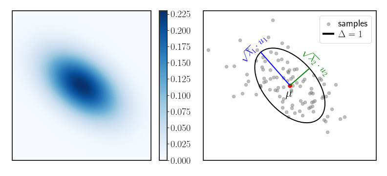
This is really clear in the 2D case:
\[\begin{equation} \Delta=\left(\frac{u_{1}^{T}\left(x-\mu\right)}{\sqrt{\lambda_{1}}}\right)^{2}+\left(\frac{u_{2}^{T}\left(x-\mu\right)}{\sqrt{\lambda_{2}}}\right)^{2} \end{equation}\]So in 2D, all of the contour lines (which are lines that have the same density along the PDF) will always be ellipses; in the multivariate case they will be ellipsoids (which is an ellipse in more dimensions, kind of). Figure 2 (right) shows this explicitly - the Gaussian is centered around the mean $\mu$ , the contour of $\Delta=1$ is an ellipse with axes aligned and scaled by the eigenvectors and square root of the eigenvalues of the covariance matrix.
Gaussians as Log-Quadratic Functions
A common approach in many probabilistic modeling methods is to ignore the normalization constant of a distribution, either because it is hard to calculate or because it’s a chore to write it down completely. Moreover, it is sometimes easier to look at distributions in log space. So, for instance, the Gaussian distribution will be written as follows: \(\begin{align} p\left(x\right) & =\underbrace{\frac{1}{Z}}_{\text{normalization}}\cdot\exp\left[-\frac{1}{2}\left(x-\mu\right)^{T}\Sigma^{-1}\left(x-\mu\right)\right]\\ \Leftrightarrow\log p\left(x\right) & =-\frac{1}{2}\left(x-\mu\right)^{T}\Sigma^{-1}\left(x-\mu\right)+\text{const} \end{align}\) where the constant term is only constant with respect to $x$ (not necessarily $\Sigma$ and $\mu$). If we open up the quadratic expression even further, we have: \(\begin{equation} \log p\left(x\right)=-\frac{1}{2}x^{T}\Sigma^{-1}x+x^{T}\Sigma^{-1}\mu+\text{const} \end{equation}\) Again, the constants are only with respect to $x$: $\mu$ is not a function of $x$, so we bunch it together with the constant terms.
So, by definition, any distribution that is log-quadratic
Derivatives of the Log-PDF
As a by-product of the above, the derivatives of the log-PDF of the Gaussian are surprisingly informative and given by: \(\begin{align} \frac{\partial}{\partial x}\log\mathcal{N}\left(x\ |\ \mu,\Sigma\right) & =\frac{\partial}{\partial x}\left[-\frac{1}{2}\left(x-\mu\right)^{T}\Sigma^{-1}\left(x-\mu\right)\right]\\ & =-\Sigma^{-1}\left(x-\mu\right) \end{align}\) This already tells us a lot. For instance, if we want to find the maximum, then we can ensure that the above equals to 0 and we get:
\[\begin{equation} -\Sigma^{-1}\left(x-\mu\right)\stackrel{!}{=}0\qquad\Leftrightarrow x=\mu \end{equation}\]since $\Sigma^{-1}\neq0$. So, we always know how to find the mean of the Gaussian distribution! We only have to find the maximum of the log-PDF.
Differentiating one more time:
\[\begin{align} \frac{\partial^{2}}{\partial x\partial x^{T}}\log\mathcal{N}\left(x\ |\ \mu,\Sigma\right) & =\frac{\partial}{\partial x^{T}}-\Sigma^{-1}\left(x-\mu\right)\\ & =-\Sigma^{-1} \end{align}\]and again we get useful information. Whenever we differentiate twice, we get the precision matrix (a different name for the inverse of the covariance).
Conditional Distribution of a Gaussian
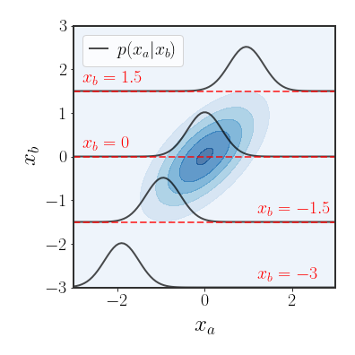
An important property of the multivariate Gaussian distribution is that if two sets of variables are jointly Gaussian, then the conditional distribution of one set on the other is also Gaussian.
Consider a Gaussian variable separated into 2 parts:
\[\begin{equation} x=\left(\begin{matrix}x_{a}\\ x_{b} \end{matrix}\right) \end{equation}\]such that $x\sim\mathcal{N}\left(\mu,\Sigma\right)$ . We can divide the mean and the covariance in a fitting manner:
\[\begin{equation} \mu=\left(\begin{matrix}\mu_{a}\\ \mu_{b} \end{matrix}\right),\quad\Sigma=\left(\begin{matrix}\Sigma_{aa} & \Sigma_{ab}\\ \Sigma_{ba} & \Sigma_{bb} \end{matrix}\right) \end{equation}\]Since the covariance is symmetrical, we know that $\Sigma_{ab}=\Sigma_{ba}^{T}$ and that $\Sigma_{aa}$ and $\Sigma_{bb}$ are symmetrical. Actually, it will be easier to use the precision matrix $\Lambda=\Sigma^{-1}$ and divide it up in the same manner:
\[\begin{equation} \Lambda=\left(\begin{matrix}\Lambda_{aa} & \Lambda_{ab}\\ \Lambda_{ba} & \Lambda_{bb} \end{matrix}\right) \end{equation}\]Full derivation to find conditional distribution
Note that $\Lambda_{aa}\neq\Sigma_{aa}^{-1}$ ! Later we will find out how each part of $\Lambda$ relates to each part of $\Sigma$ .
Let’s start by finding an expression for the conditional distribution $p\left(x_{a}\mid x_{b}\right)$ . We can find this distribution by evaluating the distribution of $p\left(x_{a},x_{b}\right)$ while fixing $x_{b}$ to a certain value and re-normalizing (the conditional distribution is a legal distribution). We will start by rewriting the quadratic term and it’s parts:
\[\begin{align} -\frac{1}{2}\left(x-\mu\right)^{T}\Lambda\left(x-\mu\right)=-\frac{1}{2}\left[\left(x_{a}-\mu_{a}\right)^{T}\Lambda_{aa}\left(x_{a}-\mu_{a}\right)\right. & +\left(x_{a}-\mu_{a}\right)^{T}\Lambda_{ab}\left(x_{b}-\mu_{b}\right)\nonumber \\ +\left(x_{b}-\mu_{b}\right)^{T}\Lambda_{ba}\left(x_{a}-\mu_{a}\right) & \left.+\left(x_{b}-\mu_{b}\right)^{T}\Lambda_{bb}\left(x_{b}-\mu_{b}\right)\right] \end{align}\]This is still a quadratic expression w.r.t. $x_{a}$ , so the conditional distribution $p\left(x_{a}\mid x_{b}\right)$ will also be Gaussian. Because the form of the Gaussian is not very flexible, as long as we find what the quadratic term is equal (the one in the exponent), the normalization will work itself out (since the conditional is also a distribution that must integrate up to 1).
We can now use the derivative trick! Defining:
\[\begin{equation} \Delta=\frac{1}{2}\left(x-\mu\right)^{T}\Sigma^{-1}\left(x-\mu\right) \end{equation}\]Starting with the first derivative:
\[\begin{equation}\label{eq:mean-form-1} \frac{\partial\Delta}{\partial x_{a}}=\Lambda_{aa}\left(x_{a}-\mu_{a}\right)+\Lambda_{ab}\left(x_{b}-\mu_{b}\right) \end{equation}\]The second derivative will give us:
\[\begin{equation} \begin{split}\frac{\partial^{2}\Delta}{\partial x_{a}\partial x_{a}^{T}} & =\Lambda_{aa}\end{split} \end{equation}\]So we know that the covariance is equal to $\Sigma_{a\mid b}=\Lambda_{aa}^{-1}$ . Using this new found knowledge, we can find the mean, if we can rewrite equation \eqref{eq:mean-form-1} as $\Lambda_{aa}\left(x_{a}-\mu_{a\mid b}\right)$ for some $\mu_{a\mid b}$ . Let’s try to do this. Recall that $\Lambda_{aa}$ is invertible, so we can write:
\[\begin{align} \Lambda_{aa}\left(x_{a}-\mu_{a}\right)+\Lambda_{ab}\left(x_{b}-\mu_{b}\right) & =\Lambda_{aa}\left(x_{a}-\mu_{a}+\Lambda_{aa}^{-1}\Lambda_{ab}\left(x_{b}-\mu_{b}\right)\right)\nonumber \\ & =\Lambda_{aa}\left[x_{a}-\left(\mu_{a}-\Lambda_{aa}^{-1}\Lambda_{ab}\left(x_{b}-\mu_{b}\right)\right)\right]\nonumber \\ & \stackrel{\Delta}{=}\Lambda_{aa}\left(x_{a}-\mu_{a\mid b}\right) \end{align}\]Which means that the conditional distribution is parameterized by:
\[\begin{align} \mu_{a\mid b} & =\mu_{a}-\Lambda_{aa}^{-1}\Lambda_{ab}\left(x_{b}-\mu_{b}\right)\\ \Sigma_{a\mid b} & =\Lambda_{aa}^{-1} \end{align}\]Okay, now all that remains is to find what $\Lambda_{aa}$ and $\Lambda_{ab}$ are equal to in terms of $\Sigma$ . To do this, we will use the following identity for partitioned matrices:
\[\begin{equation} \left(\begin{array}{cc} A & B\\ C & D \end{array}\right)^{-1}=\left(\begin{array}{cc} M & -MBD^{-1}\\ -D^{-1}CM & \quad D^{-1}+D^{-1}CMBD^{-1} \end{array}\right)^{-1} \end{equation}\]where $M=\left(A-BD^{-1}C\right)^{-1}$ is called the Schur component of the matrix with respect to the sub-matrix $D$ . Using our earlier partitioning, we get:
\[\begin{align} \Lambda_{aa} & =\left(\Sigma_{aa}-\Sigma_{ab}\Sigma_{bb}^{-1}\Sigma_{ba}\right)^{-1}\\ \Lambda_{ab} & =-\Lambda_{aa}\Sigma_{ab}\Sigma_{bb}^{-1} \end{align}\]The conditional distribution in such a setting is given by:
\[\begin{align} p\left(x_{a}\mid x_{b}\right) & =\mathcal{N}\left(x_{a}\,\mid \,\mu_{a\mid b},\Sigma_{a\mid b}\right)\\ \mu_{a\mid b} & =\mu_{a}+\Sigma_{ab}\Sigma_{bb}^{-1}\left(x_{b}-\mu_{b}\right)\nonumber \\ \Sigma_{a\mid b} & =\Sigma_{aa}-\Sigma_{ab}\Sigma_{bb}^{-1}\Sigma_{ba}\nonumber \end{align}\]Note that in this case, the conditional distribution is much easier to describe in terms of the precision matrix instead of the covariance matrix:
\[\begin{align} \mu_{a\mid b} & =\mu_{a}-\Lambda_{aa}^{-1}\Lambda_{ab}\left(x_{b}-\mu_{b}\right)\\ \Sigma_{a\mid b} & =\Lambda_{aa}^{-1} \end{align}\]When implementing the code for this, it may be simpler to save the precision matrix (as well as the covariance matrix) in memory to easily compute the conditional distribution.
Marginal Distribution of a Gaussian
Another important property of the Gaussian distribution is that its marginals are also Gaussian, which is what we will show here.
Again, we consider a Gaussian variable separated into 2 parts:
\[\left(\begin{matrix}x_{a}\\ x_{b} \end{matrix}\right)\sim\mathcal{N}\left(\left(\begin{matrix}\mu_{a}\\ \mu_{b} \end{matrix}\right),\left(\begin{matrix}\Sigma_{aa} & \Sigma_{ab}\\ \Sigma_{ba} & \Sigma_{bb} \end{matrix}\right)\right)\]and we will again define $\Lambda=\Sigma^{-1}$ . We want to find $p\left(x_{a}\right)$ .
Click here to see the derivation
Our battle plan is to first find all of the dependence on $x_{b}$ , and to integrate it out. If we can do this without losing track of $x_{a}$ , we will be able to find the marginal distribution and win. Notice that the Mahalanobis distance is quadratic in $x_{b}$ (as usual), so the final form we will get to will be something like:
\[p\left(x_{a}\right)=f\left(x_{a}\right)\intop\mathcal{N}\left(x_{b}\,\mid \,\mu_{x_{b}},\Sigma_{x_{b}}\right)dx_{b}=f\left(x_{a}\right)\]So, let’s try to open up the Mahalanobis distance (the part in the exponent) and separate it into two groups: terms that contain $x_{b}$ and those that don’t.
We begin by defining $y=x-\mu$ , which in this case will allow us to write the Mahalanobis distance as:
\[\begin{align} \Delta & =\frac{1}{2}\left(\begin{matrix}y_{a}\\ y_{b} \end{matrix}\right)^{T}\left(\begin{matrix}\Lambda_{a} & B\\ B^{T} & \Lambda_{b} \end{matrix}\right)\left(\begin{matrix}y_{a}\\ y_{b} \end{matrix}\right)\nonumber \\ & =\frac{1}{2}\left(\begin{matrix}y_{a}\\ y_{b} \end{matrix}\right)^{T}\left(\begin{matrix}\Lambda_{a}y_{a}+By_{b}\\ B^{T}y_{a}+\Lambda_{b}y_{b} \end{matrix}\right)\nonumber \\ & =\frac{1}{2}y_{a}^{T}\Lambda_{a}y_{a}+\underbrace{\frac{1}{2}\left[2y_{b}^{T}By_{a}+y_{b}^{T}\Lambda_{b}y_{b}\right]}_{\left(*\right)} \end{align}\]Note that if we find the marginal of $y_{a}$ , we effectively find the marginal of $x_{a}$ , only we don’t have to keep track of $\mu_{a}$ and $\mu_{b}$ ! We now need to complete the squares in $\left(*\right)$ to find the complete dependence on $y_{b}$ :
\[\begin{align} 2y_{b}^{T}By_{a}+y_{b}^{T}\Lambda_{b}y_{b} & =y_{b}^{T}\Lambda_{b}y_{b}+2y_{b}^{T}By_{a}\nonumber \\ & =y_{b}^{T}\Lambda_{b}y_{b}+2y_{b}^{T}\Lambda_{b}\Lambda_{b}^{-1}By_{a}\nonumber \\ & =y_{b}^{T}\Lambda_{b}y_{b}+2y_{b}^{T}\Lambda_{b}\Lambda_{b}^{-1}By_{a}+y_{a}^{T}B^{T}\Lambda_{b}^{-1}\Lambda_{b}\Lambda_{b}^{-1}By_{a}-y_{a}^{T}B^{T}\Lambda_{b}^{-1}\Lambda_{b}\Lambda_{b}^{-1}By_{a}\nonumber \\ & =\left(y_{b}+\Lambda_{b}^{-1}By_{a}\right)^{T}\Lambda_{b}\left(y_{b}+\Lambda_{b}^{-1}By_{a}\right)-y_{a}^{T}B^{T}\Lambda_{b}^{-1}By_{a} \end{align}\]We add this back to the full Mahalanobis distance to get:
\[\begin{equation} \Delta=\frac{1}{2}y_{a}^{T}\left(\Lambda_{a}-B^{T}\Lambda_{b}^{-1}B\right)y_{a}+\frac{1}{2}\left(y_{b}+\Lambda_{b}^{-1}By_{a}\right)^{T}\Lambda_{b}\left(y_{b}+\Lambda_{b}^{-1}By_{a}\right) \end{equation}\]So our distribution is:
\[\begin{align} p\left(y_{a}\right) & \propto\exp\left[-\frac{1}{2}y_{a}^{T}\left(\Lambda_{a}-B^{T}\Lambda_{b}^{-1}B\right)y_{a}\right]\intop\exp\left[-\frac{1}{2}\left(y_{b}+\Lambda_{b}^{-1}By_{a}\right)^{T}\Lambda_{b}\left(y_{b}+\Lambda_{b}^{-1}By_{a}\right)\right]dy_{b}\nonumber \\ & \propto\exp\left[-\frac{1}{2}y_{a}^{T}\left(\Lambda_{a}-B^{T}\Lambda_{b}^{-1}B\right)y_{a}\right] \end{align}\]which is definitely Gaussian! We were allowed to do the second move because the integral will be the normalization term of the Gaussian, which is a function of $\Lambda_{b}$ - which is constant with respect to $y_{a}$ (and so is eaten up by the $\propto$ sign).
Finally, we see that:
\[\begin{equation} y_{a}\sim\mathcal{N}\left(0,\left(\Lambda_{a}-B^{T}\Lambda_{b}^{-1}B\right)^{-1}\right)\Rightarrow x_{a}\sim\mathcal{N}\left(\mu_{a},\left(\Lambda_{a}-B^{T}\Lambda_{b}^{-1}B\right)^{-1}\right) \end{equation}\]and all that remains is to find what the covariance is equal to in terms of $\Sigma$ . To do this, we use the same identity we saw in the previous example:
\[\begin{equation} \Sigma_{aa}=\left(\Lambda_{aa}-B^{T}\Lambda_{b}^{-1}B\right)^{-1} \end{equation}\]So, the marginal is:
\[\begin{equation} x_{a}\sim\mathcal{N}\left(\mu_{a},\Sigma_{aa}\right) \end{equation}\]which really makes you wonder why we did all of that hard work.
The marginals of the Gaussian distribution are much more intuitive than their conditional distributions. The marginals are given by:
\[\begin{equation} x_{a}\sim\mathcal{N}\left(\mu_{a},\Sigma_{aa}\right) \end{equation}\]Extras
We saw the so called “derivative trick” and how completing the squares can also be of help, but it might not be obvious when to use each approach. First, remember that whenever we see a distribution of the form:
\[\begin{equation} p\left(x,y\right)\propto\exp\left[-x^{T}\Gamma x+b\left(y\right)^{T}x+g\left(y\right)\right] \end{equation}\]then $p\left(x\right)$ and $p\left(x\mid y\right)$ will be Gaussians
- If we don’t care about $p\left(y\right)$ or $p\left(y\mid x\right)$ at all, i.e. we want to specifically find $p\left(x\right)$ or $p\left(x\mid y\right)$ , then we can use the derivative trick
- If we need to know $p\left(y\right)$ or $p\left(y\mid x\right)$ explicitly as well as $p\left(x\right)$ or $p\left(x\mid y\right)$ , then completing the squares is usually the easiest way
- When all else fails, but we know that what we are looking for is Gaussian, we can calculate the expectations and covariance explicitly, since a Gaussian is completely defined by these two values
Once you fully understand why each method works, it will become quite clear when you should use each of them.
Discussion
Now that we know what the Gaussian distribution is and the important properties of the Gaussian distribution, we can start to use in for some real statistical problems. The next post will be dedicated to estimating $\mu$ and $\Sigma$ from observed data, after which we will move on to utilizing the Gaussian distribution in the task of regression.
← Estimation and Bayes-Optimal EstimatorsEstimating the Gaussian Distribution →