Linear Regression
Overview of the construction of linear regression as well as it's classical and Bayesian solutions.
← Estimating the Gaussian DistributionEquivalent Form →
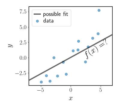
Given a vector of features $x\in\mathbb{R}^{d}$ , the simplest regression model is a function given by the weighted combination of the input features (sometimes called regressors, explanatory variables, covariates or some other name): \(\begin{equation} y=\theta_{0}+\sum_{i}\theta_{i}x_{i} \end{equation}\) where we want to predict the value of $y$ (sometimes called the response), and the $\theta$ s are the parameters of our model (sometimes called the regression coefficients). The problem of finding the $\theta$ s that estimate $y$ the best is known as linear regression
The weight $\theta_{0}$ is called the bias term, which allows the model to learn the intercept (so that $y$ doesn’t have to be 0 at $x=0$ ). We can rewrite everything in vector form by defining $x\stackrel{\Delta}{=}\left[1,x_{1},\cdots,x_{d}\right]^{T}$ and $\theta\stackrel{\Delta}{=}\left[\theta_{0},\theta_{1},\cdots,\theta_{d}\right]$ : \(\begin{equation} y=\boldsymbol{x}^{T}\boldsymbol{\theta} \end{equation}\)
Of course, we usually want to predict many $y$ s at the same time, not just one. Suppose we have $N$ feature vectors $\boldsymbol{x}_{i}\in\mathbb{R}^{d}$ (here they include the intercept term at the beginning) and a single output vector $\boldsymbol{y}\in\mathbb{R}^{N}$. We can rewrite the above for all of the outputs at once by defining:
\[\begin{equation} H\stackrel{\Delta}{=}\left[\begin{array}{ccc} - & \boldsymbol{x}_{1} & -\\ - & \boldsymbol{x}_{2} & -\\ & \vdots\\ - & \boldsymbol{x}_{N} & - \end{array}\right] \end{equation}\]Which lets us rewrite everything in the elegant form: \(\begin{equation} \boldsymbol{y}=H\boldsymbol{\theta} \end{equation}\) (from now on we will stop writing vectors in bold for ease of notation, but remember that all the variables are vectors). The matrix $H$ is sometimes called the observation matrix or the design matrix.
In the real world we usually encounter noise when sampling the function values $y$ , which we will explicitly model by adding a noise term: \(\begin{equation} y=H\theta+\eta \end{equation}\)
The noise doesn’t have to be Gaussian, but must always have zero mean. Anyway, we will model it as Gaussian for now (and this is the manner that the problem is usually presented): \(\begin{equation} \eta\sim\mathcal{N}\left(0,I\sigma^{2}\right) \end{equation}\) with $\sigma^{2}>0$. We now see that the likelihood $y\mid \theta$ is an affine transformation of a Gaussian, which is also Gaussian: \(\begin{equation} y\mid \theta\sim\mathcal{N}\left(H\theta,I\sigma^{2}\right) \end{equation}\)
Basis Functions
Notice that while the model is linear in the features $x$ , we can always define new features that are a non-linear function of $x$ , so that: \(\begin{equation} h\stackrel{\Delta}{=} h\left(x\right) \end{equation}\) where $h:\mathbb{R}^{d}\rightarrow\mathbb{R}^{p}$. The solution to the linear regression problem defined above will of course be linear in $h$, but will not be linear in the original features $x$ . In this case, we would say that we have $p$ basis functions such that: \(\begin{equation} h=h\left(x\right)=\left[h_{1}\left(x\right),h_{2}\left(x\right),...,h_{p}\left(x\right)\right]^{T} \end{equation}\) and each $h_{i}\left(\cdot\right)$ is called a basis function and has the form of $h_{i}:\mathbb{R}^{d}\rightarrow\mathbb{R}$ .
Common Basis Functions
Polynomial basis functions (PBF) are the simplest kind of basis functions we will see in the course. In these basis functions, the features are powers of the input variables $x$ up to a certain degree. For instance, if: \(x=\left[\begin{array}{c}x_{1}\\x_{2}\end{array}\right]\) then the features for a PBF of degree 2 are $1,\,x_{1},\,x_{2},\,x_{1}^{2},\,x_{1}x_{2},\,x_{2}^{2}$ . For degree 3, we would add $x_{1}^{3},\,x_{1}^{2}x_{2},\,x_{1}x_{2}^{2},\,x_{2}^{3}$ and so on for any degree we want to use. These are called polynomial basis functions since the form $\theta^{T}h\left(x\right)$ for degree $q$ describes a polynomial function of degree $q$ (polynomial in $x$ ).
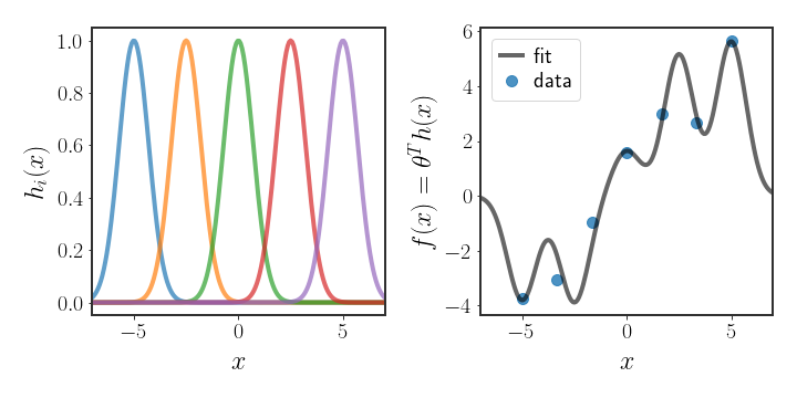
Another commonly used basis function is: \(\begin{equation} h_{j}\left(x\right)=\exp\left[-\frac{\mid\mid x-\mu_{j}\mid\mid ^{2}}{2s^{2}}\right] \end{equation}\) which is called, for obvious reasons, the Gaussian basis function. Note that while this basis function is related to the Gaussian distribution, it doesn’t need to be a proper distribution. One way to use the Gaussian basis function is to decide, ahead of time, where $K$ different centers $\mu_{j}$ will be placed, and use the distances from each of them as the features. This has the obvious limitations that we are the ones that chose where the centers should be placed, and so they may not be optimal for the data. An example use case of such basis functions is given in figure (2); notice how the learned function has hills and valleys corresponding to the locations of the basis functions.
Of course, there are many more possible basis functions that can be used. Since there are many possible basis functions and some may work better than others on our data, we may run into issues of how to choose the best model. Later on we will discuss how to select which basis function to use from the myriad possibilities, but for now we will ignore this problem, since the optimization process for linear regression doesn’t depend on the specific basis function that is used.
Classical Linear Regression
In the classical formulation of linear regression, the ML estimate for $\theta$ is used to define the function $y\left(x\right)$ . Let’s find this estimate. First, let’s write out the log-likelihood explicitly: \(\begin{align} \ell\left(y\,\mid \,\theta\right) & =\sum_{i=1}^{N}\log\mathcal{N}\left(y_{i}\,\mid \,h\left(x_{i}\right)^{T}\theta,I\sigma^{2}\right)\nonumber \\ & =-\frac{1}{2\sigma^{2}}\sum_{i=1}^{N}\mid\mid y_{i}-h\left(x_{i}\right)^{T}\theta\mid\mid ^{2}+\text{const}\\ & =-\frac{1}{2\sigma^{2}}\mid\mid y-H\theta\mid\mid ^{2}+\text{const} \end{align}\) where we will ignore terms that are constant with respect to $\theta$ for now. Finding the maximum of this log-likelihood is often called least squares as we are trying to minimize a sum of square functions over $\theta$ ; the function we are trying to maximize is the negative of the loss: \(\begin{equation} L=\frac{1}{2}\mid\mid y-H\theta\mid\mid ^{2} \end{equation}\)
We can differentiate the log-likelihood by $\theta$ and equate to 0 to find the minimum (the function is quadratic, so the only stationary point is the minimum): \(\begin{equation} \frac{\partial}{\partial\theta}L=H^{T}\left(H\theta-y\right)\stackrel{!}{=}0 \end{equation}\) \(\begin{align} H^{T}H\theta & =H^{T}y\\ \Rightarrow\hat{\theta}_{ML} & =\left(H^{T}H\right)^{-1}H^{T}y \end{align}\)
Geometry of Least Squares
We can gain further insight into the ML solution by looking at the geometry of the least squares solution
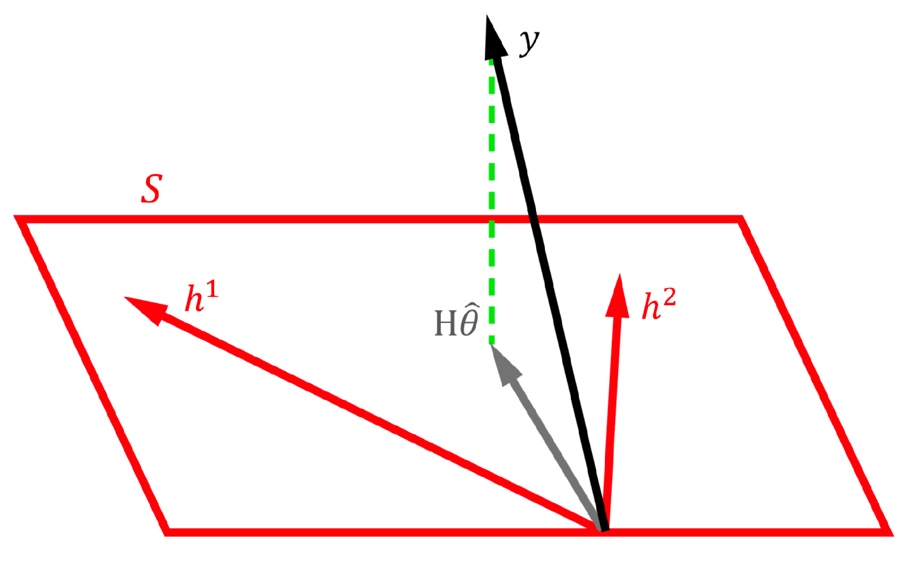
Let’s look at the $N$ dimensional vector $y=\left(y_{1},y_{2},…,y_{N}\right)^{T}$ and the columns of $H$ , which we will denote as $h^{\left(j\right)}$ for now. Some subspace $\mathcal{S}$ is spanned by the $d$ column vectors in $H$ , which leaves us with three possible scenarios that we have to think about when talking about the ML solution $\hat{\theta}_{\text{ML}}=\left(H^{T}H\right)^{-1}H^{T}y$ :
- There exists some $\theta$ such that $H\theta=y$ exactly
- $y$ is in the orthogonal complement of $\mathcal{S}$, i.e. $H^{T}y=0$
- $y$ is a combination of the above two scenarios, in which case we can rewrite it as a part that lies in the subspace plus an orthogonal part: $y=y_{\mathcal{S}}+y_{\perp}\stackrel{\Delta}{=} H\theta_{\mathcal{S}}+y_{\perp}$
Plugging this into the least squares solution, the prediction $\hat{y}$ that we will make is:
\[\begin{align*} \hat{y} & =H\hat{\theta}_{\text{ML}}=H\left(H^{T}H\right)^{-1}H^{T}y\\ & =H\left(H^{T}H\right)^{-1}H^{T}\left(H\theta_{\mathcal{S}}+y_{\perp}\right)\\ & =H\left(H^{T}H\right)^{-1}H^{T}H\theta_{\mathcal{S}}+H\left(H^{T}H\right)^{-1}H^{T}y_{\perp}\\ & =H\theta_{\mathcal{S}}=y_{\mathcal{S}} \end{align*}\]The geometrical interpretation of the above is that $H\hat{\theta}_{ML}$ is the projection of $y$ onto $\mathcal{S}$ , the subspace that the basis functions in $H$ are able to span. You may find it easier to see this visually as in the figure below:
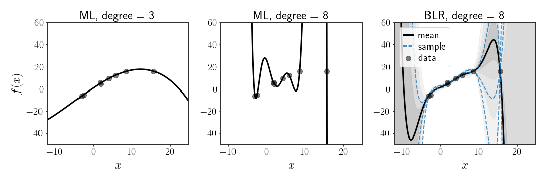
While very simple, the ML solution for linear regression is prone to problems. Specifically, notice that when the basis functions are expressive enough to completely fit the points, then they will always do so, even when we might think that such a solution doesn’t make much sense. This is called overfitting and can be seen in figure 4 below (center). In fact, this will happen whenever the basis functions span a subspace with the same rank as the number of data points. When this subspace has a larger rank than the number of points, then there are an infinite number of solutions!
Ridge Regression
As we add more and more basis functions, we will start overfitting at some point - something we would really like to avoid. Regularization seeks to reduce the amount of overfitting by adding some restrictions to the values that the weights can take. Usually this is done by adding a penalty term for $\theta$ to what we are trying to minimize, like so:
\[L_{R}=\frac{1}{2}\mid\mid y-H\theta\mid\mid ^{2}+\lambda E_{R}\left(\theta\right)\]where $\lambda$ is the regularization coefficient that controls the relative weight between the least squares expression and the regularization penalty $E_{R}$ . The simplest form of regularization is given by the norm of the weights: \(\begin{equation} E_{R}\left(\theta\right)=\frac{1}{2}\theta^{T}\theta=\frac{1}{2}\mid\mid \theta\mid\mid ^{2} \end{equation}\) Adding this term to the least squares objective the loss function becomes: \(\begin{equation} L_{R}=\frac{1}{2}\mid\mid y-H\theta\mid\mid ^{2}+\frac{\lambda}{2}\mid\mid \theta\mid\mid ^{2} \end{equation}\) This is only one possible choice for regularization, but is useful since it’s easy to find the optimal solution with this regularization. Minimizing $L_{R}$ with respect to $\theta$ , we get: \(\begin{equation}\label{eq:ridge-sol} \hat{\theta}=\left(H^{T}H+I\lambda\right)^{-1}H^{T}y \end{equation}\) Linear regression with this regularization is often called ridge regression. This type of regularization obviously adds more constraints to the optimal values of $\theta$ since the weights are penalized based on their magnitude, unlike before. Another way to think about this is that $\lambda$ suggests a certain budget that the whole model gets for fitting the weights - if $\mid\mid y-H\theta\mid\mid ^{2}$ is constant and we change the value of $\lambda$ , then it directly controls the total magnitude of $\theta$ .
Bayesian Linear Regression
Of course, we can also have a prior over the parameters $\theta$
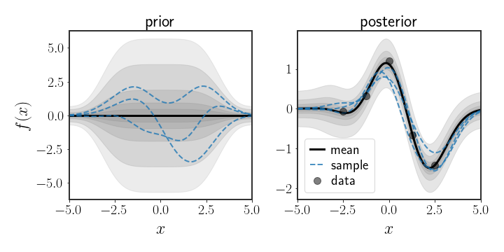
The posterior $p\left(\theta\mid y\right)$ in this case is also a Gaussian distribution given by
The optimal estimator (in the BMSE sense), as we have previously seen, is given by the expectation of the posterior: \(\begin{equation} \mathbb{E}\left[\theta\mid D\right]=C_{\theta\mid D}\left(H^{T}\frac{1}{\sigma^{2}}y+\Sigma_{\theta}^{-1}\mu_{\theta}\right) \end{equation}\)
Connection to Classic Linear Regression
Since our posterior is a Gaussian, the MMSE and MAP estimates coincide, so let’s look at $\mathbb{E}\left[\theta\mid y\right]$ when the prior is non-informative; this will show us how the MMSE and ML solutions are related. We can do so by defining: \(\begin{equation}\label{eq:ridge-prior} \theta_{R}\sim\mathcal{N}\left(0,\alpha I\right) \end{equation}\) At the limit $\alpha\rightarrow\infty$, this prior becomes closer and closer to uniform on the whole space. Using this prior, the expectation over the posterior becomes: \(\begin{align} \mathbb{E}\left[\theta_{R}\mid y\right] & =\left(I\frac{1}{\alpha}+\frac{1}{\sigma^{2}}H^{T}H\right)^{-1}H^{T}\frac{1}{\sigma^{2}}y\nonumber \\ & =\sigma^{2}\left(I\frac{\sigma^{2}}{\alpha}+H^{T}H\right)^{-1}H^{T}\frac{1}{\sigma^{2}}y\nonumber \\ & =\left(I\frac{\sigma^{2}}{\alpha}+H^{T}H\right)^{-1}H^{T}y\label{eq:bayes-ridge}\\ & \stackrel{\alpha\rightarrow\infty}{=}\left(H^{T}H\right)^{-1}H^{T}y \end{align}\) And we have the MLE solution! But wait, we didn’t do that just for show. If we rewind back to equation \eqref{eq:bayes-ridge}, notice that this looks suspiciously similar to equation \eqref{eq:ridge-sol}, where we saw the solution to ridge regression. Now we can give a more informative explanation to ridge regression; instead of saying something a bit hand wavey as “we are trying to avoid overfitting”, we can say that ridge regression is the same as Bayesian linear regression with a prior of the form given in equation \eqref{eq:ridge-prior}. Equivalently, using $\theta_{R}$ as a prior is like trying to solve ridge regression with the regularization: \(\begin{equation} \lambda=\frac{\sigma^{2}}{\alpha} \end{equation}\) In this sense, if we are very unsure about the prior ( $\alpha\gg1$ ) then the regularization will be very light, while if we are very sure ( $\alpha$ is small), then we will heavily penalize solutions that are far from what we expected.
Discussion
We have finally made it to the first “real” example of machine learning in this collection of posts. Linear regression seems like a really simple model but therein lies its’ strengths. It’s east to understand the predictions by the linear regression model and tweaking the basis functions allows for a ton of versatility. By moving to Bayesian linear regression, we can get a sense of uncertainty in the prediction of the model, which is a pretty attractive attribute.
In the next post, we will see a different form for writing the solution to Bayesian linear regression which is sometimes used in literature. In the post after, we will look into ways to choose which basis functions to use given some observations.