Annealed Importance Sampling
Suppose you can’t find your keys. You know you left them in your apartment somewhere, but don’t remember where. This happens pretty often, so you have a keep note of the possible places you may have left your keys. You want to find out the probability that the keys are in a specific room of your apartment. Let’s call this room $R$ - mathematically speaking, you want to calculate: \(\begin{equation} P\left(\text{keys}\in R\right)=\intop \mathbf{1}\left[x\in R\right]\cdot p_\text{keys}(x)dx \end{equation}\)
where $x\in\mathbb{R}^2$ is a two-dimensional coordinate where the keys may have been forgotten and $p_\text{keys}(x)$ is the PDF for the keys to be in the location $x$. The function $\mathbf{1}\left[x\in R\right]$ equals 1 if $x\in R$, otherwise it is 0. The above can be rewritten:
\[\begin{equation} P\left(\text{keys in }R\right) = \mathbb{E}_{x\sim p_\text{keys}}\left[\mathbf{1}\left[x\in R\right]\right] \end{equation}\]So… how can we calculate (or approximate) this expectation? Which room is most probable to contain your lost keys?
While this example is a bit silly, the problem can be abstracted to fit many different situations. In this post, I’m going to show how it can be solved using Annealed Importance Sampling (AIS,
Problem Statement
Let’s define the problem again, just a bit more generally.
We have some distribution over the domain $\mathcal{X}$: \(\begin{equation} p(x)= \frac{1}{Z}\tilde{p}(x) \end{equation}\)
where for a given $x$ we know how to calculate $\tilde{p}(x)$. In this example, I’m going to assume the normalizing constant $Z$ isn’t known. This setting matches a situation where you keep track of where the keys were left in the past and have a non-parametric formulation for the density $\tilde{p}(x)$, in which case $Z$ is hard to calculate.
I will also assume that there’s a function $f:\mathcal{X}\rightarrow \mathbb{R}$ and we want (for whatever reason) to calculate:
\[\begin{equation}\label{eq:f-exp} \overline{f}=\mathbb{E}_{x\sim p(x)}\left[f\left(x\right)\right] \end{equation}\]In our example, $p(x)=p_\text{keys}(x)$ and $f(x)=\mathbf{1}\left[x\in R\right]$.
The question is: how can we calculate $\overline{f}$? And as a secondary goal: is there a way to estimate $Z$ simultaneously, so we have access to the full (normalized) distribution?
First Approach
One way to find $\overline{f}$ and $Z$ is using importance sampling (IS). In IS, a simple distribution $q(x)$ is chosen and the expectation in equation \eqref{eq:f-exp} is approximated according to (see A.1 for more details):
\[\begin{equation} \tilde{w}(x)=\frac{\tilde{p}(x)}{q(x)}\qquad\overline{f}\approx \frac{\sum_{x_i\sim q}\tilde{w}(x_i)f(x_i)}{\sum_{x_i\sim q}\tilde{w}(x_i)} \end{equation}\]The number $\tilde{w}(x)$ defines the relative importance of $x$ under our distribution of interest $\tilde{p}(x)$ and the simple distribution $q(x)$, which is why $\tilde{w}(x)$ are called importance weights.
IS also let’s us approximate the normalization constant $Z$, using only the importance weights: $Z=\mathbb{E}q\left[\tilde{w}(x)\right]\approx\frac{1}{N}\sum{x_i\sim q}^N\tilde{w}(x_i)$.
This seems to solve the problem we defined earlier. Of course, this post is about annealed IS, not IS, so there’s going to be a bit more to read.
While incredibly simple and easy to use, IS is actually pretty hard to calibrate. Here, calibration means choosing a distribution $q(x)$ that is similar in some sense to $p(x)$. The best we can do, after all, is $q(x)=p(x)$. In that case, all of the importance weights will be equal to 1 and we would get a perfect approximation of $\overline{f}$ and $Z$. No, usually a much simpler distribution $q(x)$ is chosen, and if $q(x)\gg p(x)$ in some region of space then many samples from $q(x)$ will end up with very low importance weights $\tilde{w}(x)$. In such a situation, an enormous number of samples has to be used in order to get a sound approximation.
Another Way
If we are solely interested in estimating the expectation in equation \eqref{eq:f-exp}, then another alternative is available - as long as we have some method for producing samples from $p(x)$ using only the unnormalized function $\tilde{p}(x)$. If that is the case, then $M$ points $x_1,\cdots,x_M$ can be sampled and used to get an unbiased approximation of the expectation:
\[\begin{equation} \overline{f}\approx\frac{1}{M}\sum_{i:\ x_i\sim p}^M f(x_i) \end{equation}\]To this end, Markov chain Monte Carlo (MCMC) methods can be used, such as Langevin dynamics, in order to sample from the distribution. Many of these MCMC methods only require access to the gradient of the log of the distribution, $\nabla \log p(x)=\nabla \log \tilde{p}(x)$, so not knowing the normalization constant isn’t a problem. However, this doesn’t give us any estimate of $Z$ and many times it’s also difficult to tune an MCMC sampler.
Combining IS with MCMC
At it’s core, AIS is a way to combine the importance weights in IS with an MCMC approach. The idea is relatively simple: start with a sample from a simple distribution $q(x)$ and use MCMC iterations to get this sample closer to the distribution of interest $p(x)$. At the same time, we can also keep track of the relative importance of the sample, getting better calibrated importance weights.
That’s the main intuition behind AIS. Don’t worry if it’s still unclear, you have a bit more to read which I hope will clarify things.
Annealing the Importance Distribution
As in IS, we begin by choosing: \(\begin{equation} q(x)=\frac{1}{Z_0}\tilde{q}(x) \end{equation}\) which is easy to sample from and whose normalization constant, $Z_0$, is known.
How are we going to get this sample closer to $p(x)$? We’re going to define a series of intermediate distributions that gradually get closer and closer to $p(x)$. For now I’ll define the $T$ intermediate distributions as:
\[\begin{aligned} \pi_t(x)&=\tilde{q}(x)^{1-\beta(t)}\cdot\tilde{p}(x)^{\beta(t)}\\ \beta(t)&=t/T \end{aligned}\]where $p(x)=\tilde{p}(x)/Z_T$ is the distribution we’re actually interested in. Notice that $\beta(0)=0$ and $\beta(T)=1$, so:
\[\begin{align} \pi_0(x)&=\tilde{q}(x)\\ \pi_T(x)&=\tilde{p}(x) \end{align}\]Furthermore, the values of $\beta(t)$ gradually move from 0 to 1, so for each $t$ the function $\pi_t(x)$ is an unnormalized distribution somewhere between the two distributions $\tilde{q}(x)$ and $\tilde{p}(x)$. These intermediate distributions will allow a smooth transition from the simple distribution to the complex.
If we use many iteration $T$, then the difference between each $\pi_t(x)$ and $\pi_{t+1}(x)$ will be very small, such that a sample from $\pi_t(x)$ is almost (but not quite) a valid sample from $\pi_{t+1}(x)$. Accordingly, we can use a relatively lightweight MCMC approach to get a sample from $\pi_{t+1}(x)$ starting from the $\pi_t(x)$ sample. And we can do this for all $t$, starting from the initial simple distribution $\pi_0(x)$.
At the same time, the importance weights for $\pi_{t+1}(x)$ given the $\pi_t(x)$ “proposal distribution” are $w_t=\frac{\pi_{t+1}(x)}{\pi_{t}(x)}$. We essentially want to get the importance weights for the whole chain $\pi_0(x)\rightarrow \pi_1(x)\rightarrow\cdots\rightarrow \pi_T(x)$, so we will multiply the time-based importance weights along the way. Ultimately, given a chain of $x_0,\cdots,x_{T-1}$ the importance weight of the whole chain will be given by:
\[\begin{equation} w(x_0,\cdots,x_T)=Z_0\frac{\pi_1(x_0)}{\pi_0(x_0)}\cdot\frac{\pi_2(x_1)}{\pi_1(x_1)}\cdots \frac{\pi_T(x_{T-1})}{\pi_{T-1}(x_{T-1})} \end{equation}\]Notice that for all the intermediate $t$s that are not equal to 0 or $T$, the unnormalized distribution $\pi_t(x)$ always appears in the numerator and denominator once, meaning that we don’t need to estimate the normalizing coefficients $Z_t$ as they cancel out.
Putting all of this together, the AIS algorithm proceeds as follows (see appendix A.2 for something a bit more formal):
- sample $x_0\sim q(x)$
- set $w_0=Z_0$
- for $t=1,\cdots,T$:
- $\qquad$set $w_t=w_{t-1}\cdot\frac{\pi_t(x_{t-1})}{\pi_{t-1}(x_{t-1})}$
- $\qquad$sample $x_t\sim \pi_t(x)$ starting from $x_{t-1}$
That’s it.
Small Notes
For this post, I chose a particular (“standard”) way to define the intermediate distributions $\pi_t(x)$. However, any set of intermediate distributions can be chosen, as long as the unnormalized form of each of them can be calculated and the change is gradual enough.
Additionally to that, while $\pi_t(x)=\pi_0^{1-\beta(t)}(x)\pi_T^{\beta(t)}(x)$ is the definition most often used in practice, $\beta(t)$ is usually not just linear in $t$. There are many options for the scheduling/annealing of $\beta(t)$, where different heuristics are taken into account in the definition of the schedule.
Examples and Visualizations
Implementation details
In all of the following examples, I’m using Langevin dynamics or the Metropolis corrected version (called MALA) with a single step as the MCMC algorithm between intermediate distributions. Moreover, I always used $q(x)=\mathcal{N}(x;\ 0, I)$ as the proposal distribution.
To be honest, this would not work in any real application - a single Langevin step doesn’t sample from the distribution (you usually need many more steps). Luckily, for these visualizations a single step was enough and conveys the message equally well, so I’d rather keep the simpler approach for now.
The first example is really simple - the target and proposal distributions are both Gaussian:

An important advantage of AIS is that it anneals between a simple distribution, slowly morphing into the more complicated distribution. If properly calibrated, this allows it to sample from all modes:
Of course, AIS can be used to sample from much more complex distributions:
Importance Weights
The mathematical trick of AIS is the way we defined the weights, $w_T$ (see A.2 for more details regarding the definition). Like in regular importance sampling, the weights are defined in such a way that:
\[\begin{equation} \mathbb{E}_{x_0\sim q}\left[w_T\right]=Z_T \end{equation}\]So, we can use $M$ samples $x_T^{(1)},\cdot,x_T^{(M)}$ and importance weights $w_T^{(1)},\cdots,w_T^{(M)}$ created using the AIS algorithm to estimate the expectation from equation \eqref{eq:f-exp}:
\[\begin{equation} \overline{f}\approx\hat{f}= \frac{\sum_i^M w_T^{(i)}f(x_T^{(i)})}{\sum_i^M w_T^{(i)}} \end{equation}\]In fact, this $\hat{f}$ is an unbiased estimator for $\overline{f}$!
Calculations in Log-Space
If you’ve ever dealt with probabilistic machine learning, you probably already know that multiplying many (possible very small) probabilities is a recipe for disaster. This is also true here.
Recall:
\[\begin{equation} w_T=Z_0\cdot\frac{\pi_1(x_0)}{\pi_0(x_0)}\cdot\frac{\pi_2(x_1)}{\pi_1(x_1)}\cdots\frac{\pi_T(x_{T-1})}{\pi_{T-1}(x_{T-1})} \end{equation}\]In almost all practical use cases, the values $\pi_i(x)$ are going to be very small numbers. So, $w_T$ is the product of many small numbers. If $T$ is very large, it is almost guaranteed that the precision of our computers won’t be able to handle the small numbers and eventually we’ll end up with $w_T=0/0$.
Instead, the importance weights are usually calculated in log-space, which modifies the update for the importance weight into:
\[\begin{equation} \log w_t=\log w_{t-1}+\log \pi_t(x_{t-1})-\log\pi_{t-1}(x_{t-1}) \end{equation}\]The log-weights can then be averaged to get an estimate of $\log Z_t$… well, almost.
Averaging out the log-weights gives us $\mathbb{E}_{x_0\sim q(x)}[\log w_T]$ , however by Jensen’s inequality
So, when we use the log of importance weights, it’s important to remember that they only provide us with a stochastic lower bound
Bottom line is: the number of intermediate distributions $T$ should be quite large and carefully calibrated.
Reversing the Annealing
There is a silver lining to the above. If we reverse the AIS procedure, that is start at $\pi_T(x)$ and anneal to $\pi_0(x)$, then we can generate a stochastic upper bound of $Z_T$.
Keeping the same notation as above, let $w_T$ be the importance weights of the regular AIS and $m_0$ be the importance weights of the reverse annealing. Then:
\[\begin{align} \mathbb{E}_{x_T\sim p}[\log m_0]&\le \log \mathbb{E}_{x_T\sim p}[m_0]=\log\frac{1}{Z_T}\\ \Leftrightarrow \log Z_T&\ge - \mathbb{E}_{x_T\sim p}[\log m_0] \end{align}\]The only problem, which you may have noticed, is that the reverse procedure needs to start from samples out of $p(x)$, our target distribution. Fortunately, such samples were produced by the forward procedure of AIS
Finding Your Keys
Back to our somewhat contrived problem.
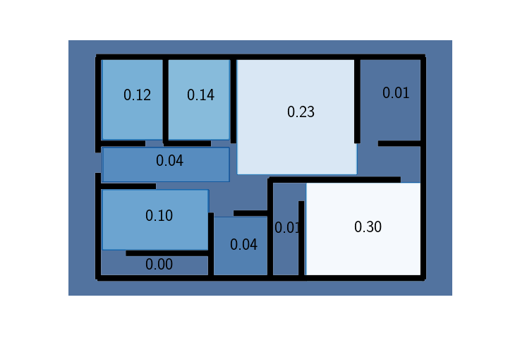
Here’s your apartment and the PDF for $p_\text{key}(x)$ representing the distribution of probable key placements:
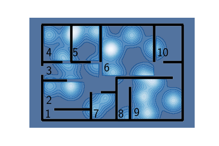
Your place is really big
As you can see, there are rooms more likely and less likely to contain the keys and there are regions where it would be almost impossible to find the keys (all the places with the darkest shade of blue). Such places are, for instance, outside the house, in the walls or in the middle of a hallway.
Conveniently, the rooms are numbered. We want to estimate, given this (unnormalized) PDF the probability that the keys are in a room, say room 7:
\[\begin{equation} P(\text{keys}\in R_7)=? \end{equation}\]Well, let’s use AIS to calculate the importance weights. Here’s the compulsory animation:
More implementation details
Unlike the previous animations, for these trajectories I actually used 100 samples and am only showing 30 (otherwise everything would be full of moving black dots). Also, notice that towards the end of the AIS procedure the particles get “stuck”; this is because I used Metropolis-Hastings acceptance steps
Also, the annealing for this animation was a bit tricky to set. Because the density outside the house is basically constant (and equal to 0), if the annealing isn’t carefully adjusted points have a tendency of getting stuck there. My solution was to also anneal the impossibility of being in those regions, just in a much slower pace than the other parts of the distribution
Using the importance weights accumulated during this sampling procedure, we can now calculate the probability of the keys being in any one of the rooms, for instance room 7:
\[\begin{align} P(\text{keys}\in R_7)&=\mathbb{E}_x\left[\textbf{1}[x\in R_7]\right]\\ &\approx\frac{\sum_i w_T^{(i)}\cdot \textbf{1}[x\in R_7]}{\sum_i w^{(i)}_T} \end{align}\]Using this formula to calculate the probabilities of the keys being in each of the rooms, we get:
And there you have it! You should probably check in either room 9 or 6 and only then search in the other rooms.
Practical Applications of AIS
While I believe the example in this post is good for visualization and intuition, it’s pretty silly (as I already mentioned). In 2D, rejection sampling probably achieves the same results with much less fuss.
The more common use for AIS that I’ve seen around is as a method for Bayesian inference (e.g.
Suppose we have some prior distribution $p(\theta;\ \varphi)$ parametrized by $\varphi$ and a likelihood $p(x\vert\theta)$. Bayesian inference is, at it’s core, all about calculating the posterior distribution and the evidence function:
\[\overbrace{p(\theta\vert x;\varphi)}^\text{posterior}=\frac{p(\theta)\cdot p(x\vert \theta)}{\underbrace{p(x;\varphi)}_\text{evidence}}\]For most distributions in the real world this is really really hard. As a consequence, using MCMC methods for sampling from the posterior (or posterior sampling) is very common. However, such methods don’t allow for calculation of the evidence, which is one of the primary ways models are selected in Bayesian statistics.
AIS offers an elegant solution both to posterior sampling and evidence estimation. Let’s define our proposal and target distributions once more, adjusted for Bayesian inference:
\[\begin{equation} \pi_0(\theta)=p(\theta;\ \varphi)\qquad\ \ \ \ \ \ \ \ \pi_T(\theta)=p(\theta;\varphi)\cdot p(x\vert\ \theta) \end{equation}\]As you have probably already noticed, $\pi_T(\theta)$ is the unnormalized version of the posterior. The normalization constant of $\pi_T(\theta)$ is exactly the evidence. We only need to choose an annealing schedule between the proposal and target distributions. Taking inspiration from our earlier annealing schedule, we can use (for example):
\[\begin{equation} \pi_t(\theta)=p(\theta;\varphi)\cdot p(x\vert\theta)^{\beta(t)} \end{equation}\]where $\beta(0)=0$ and $\beta(T)=1$.
That’s it. If $T$ is large enough, then we can be sure that the samples procured from the AIS algorithm will be i.i.d. from the posterior. Moreover, the weights $w_T^{(i)}$ can be used to estimate the evidence:
\[\begin{equation} p(x;\varphi)\approx \frac{1}{M}\sum_i w_T^{(i)} \end{equation}\]And there you have it! Instead of simply sampling from the posterior, you can get an estimate for the evidence at the same time
Conclusion
You now (maybe) know what annealed importance sampling is and how to use it. My main hope was to give some intuition into what happens in the background when you use AIS. I find the concept of sampling by starting at a simple distribution and moving to a more complex one really cool, especially when it is treated in such a clear and direct manner.