A Simplified Overview of Langevin Dynamics

An overview of Langevin dynamics (or sampling), with a focus on building up intuition for how it works, when it works, and what can be done to make it work when it doesn't.

Langevin dynamics (or sampling) is one of the most popular Markov chain Monte Carlo (MCMC) methods out there. It is used for countless tasks that require sampling from a distribution, and is even really simple to use especially since automatic differentiation is easily accessible. While straightforward to implement, I think that it’s hard to build an intuition for what to expect without seeing toy examples. In this post, I want to try and build the intuition for the sampling procedure itself, the stationary distribution that will be reached, and how to mitigate possible problems with the sampling procedure.

Problem Setting

Suppose we have the following distribution:

\[\begin{equation}\label{eq:prob} p(x)\propto e^{-f(x)}\Leftrightarrow \log p(x)=-f(x)+\text{const} \end{equation}\]

where $x\in\mathbb{R}^d$ and $f(x)$ is some function so that the integral $\intop e^{-f(x)}dx$ doesn’t diverge (i.e. $p(x)$ is a valid distribution).

We would like to sample from this distribution, but don’t have any way to do so directly. Worse, we don’t know the conditional or marginal distributions under this PDF, so we can’t use methods such as Gibbs sampling. However, what we do know is the gradient of the function at every point: $\nabla f(x)$ The function $f(x)$ is sometimes called the energy function and the negative gradient the potential function.

While we don’t know the distribution itself, we obviously know quite a bit about the distribution if we know how to differentiate it. Specifically, we can use gradient descent (GD) in order to find the modes of the distribution:

\[\begin{equation} x_t=x_{t-1} - \eta_t \nabla f(x_{t-1}) \end{equation}\]

where $\eta_t > 0$ is a scalar usually called the learning rate or step size. If we can find the modes of the distribution, then it follows that we can find the areas with peaks in the density, i.e. areas which may be quite likely in the distribution. So while we may not know the distribution itself (only an unnormalized function that defines the distribution), the gradients actually tell us quite a bit about the function.

Langevin sampling, which will be introduced in the next section, looks like a weird modification of GD. We will see that it amounts to adding noise every iteration of the GD algorithm. An easy (but not entirely correct) way to start thinking about Langevin sampling is that if we add some kind of noise to each step of the GD procedure, then most of the time the chain will converge to areas around the biggest peaks, instead of arriving at a local maxima of the distribution.

Langevin Sampling

As I mentioned, the sampling algorithm is surprisingly simple to implement and is iteratively defined as:

\[\begin{equation}\label{eq:langevin} x_{t+1}=x_t - \frac{\epsilon}{2}\nabla f(x_t)+\sqrt{\epsilon}\mathcal{N}\left(0,I\right) \end{equation}\]

where $\epsilon>0$ is a (small) constant.

Let’s look at a simple example of this in action:

Figure 1: an example of a single chain of Langevin sampling from a (simple) Gaussian distribution. The brighter areas denote areas with higher probabilities while the black dot is the sample in the current iteration. The trailing dots are previous iterations, which fade out gradually.

As you can see, the little dot (which follows $x_t$ though the iterations) moves around in the bright areas of the distribution. Sometimes it explores outside of the bright regions, only to return. In general, the whole distribution is explored pretty quickly , as we would want it to be.

Convergence

Using the update rule of equation \eqref{eq:langevin}, the sample $x_T$ will converge to a sample from the distributionUnder some reasonable (but needed) assumptions over $f(\cdot)$ in equation \eqref{eq:prob} at the limit $T\rightarrow \infty$ and $\epsilon \rightarrow 0$ . Obviously, we can’t wait an infinite number of time steps, so usually $T$ and $\epsilon$ are tuned by hand so that $T$ is “large enough” and $\epsilon$ is “small enough”. Convergence in this sense means that if we have many points that are initialized from the same point, after a long enough time $T$ , we would be able to approximate the distribution with these samples; the follow gives a small example of this:

Figure 2: the left side shows the true distribution and 100 points sampled according to Langevin from this distribution, while the plot on the right shows the approximated distribution according to 1000 sampled points. Notice how the distribution is very different from the true one at the beginning, after which it slowly gets closer and closer to the true distribution.

---

Usually each function we want to sample from requires different handling. Notice how in figure 1 it seems like ~200 steps are enough to reach a sample from the distribution. Now, let’s look at a slightly slower example:

Figure 3: another example of a single chain of Langevin sampling, only on a narrower Gaussian. While the chain reaches the bright part of the distribution quite quickly, it always remains in the top half (for all 800 iterations).

The chain arrives at the distribution fast enough, but then stays in the upper half of the distribution for it’s whole life time - for 800 iterations! This means that if we want to sample two points , which are initialized close to each other, then they will probably be very close to each other even after 800 iterations. In MCMC terms, we would say that the chain hasn’t mixed yet. This is in contrast to the example in figure 1, where ~200 iterations are enough for the chain to mix.

In this case, intuition calls for a very simple modification - change the step size! If we increase the step size, then the dot would move further each iteration, and the chain would “mix” very rapidly, right? However, finding the right value for $\epsilon$ is actually pretty difficult. Consider the following toy example:

Figure 4: an example of bad settings of $\epsilon$. On the left, you can see the distribution and true samples from it. The middle two images show what happens when $\epsilon$ is too large (left) and too small (right). The right-most graph shows the average negative log-likelihood (the average value of $f(x)$ ) for each of the images to the left of it.

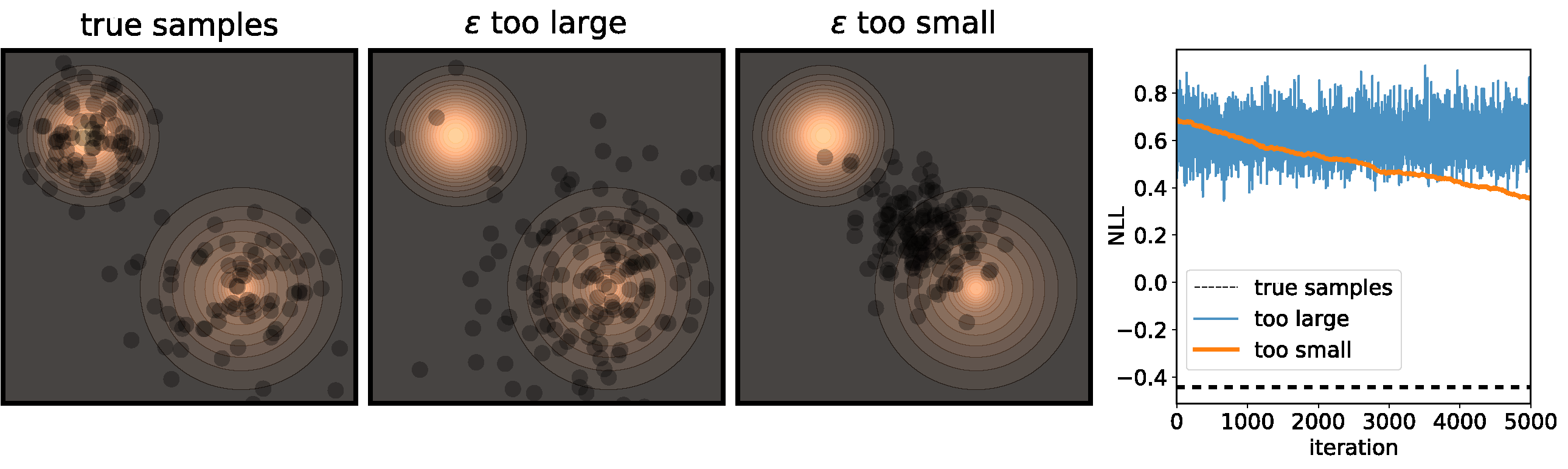
Figure 3 illustrates the problems that can happen if $\epsilon$ isn’t correctly calibrated. If it is too large, then we’re adding a bunch of noise each iteration, so while the chain will converge at its’ stationary distribution very quickly, the stationary distribution will be very different from the distribution we actually want to sample from. On the other end of the spectrum, if $\epsilon$ is too small then it will take a very long time for the samples to move from their initial positions.

Okay, so forget about getting there quickly, let’s just run a chain for very very long - that should be fine, right?

Not really. Up until now I only showed examples where the distribution is mostly gathered together. Let’s see what happens when there are two separated islands:

Figure 5: what happens if the distribution is separated into islands? On the left you can see the true distribution as well as 100 Langevin chains running. On the right is a visualization of the distribution that 1000 Langevin chains approximate.

If we use a small $\epsilon$ when there are islands in the distribution, then Langevin might converge to a good representation of one of the islands, but the samples won’t “hop” between the islandsIf we wait long enough, they will. But as you can see above, in the 2000 iterations, only one dot from the 1000 made it across.. On the other hand, if $\epsilon$ is large, then both islands might be well represented by the samples, but the approximated distribution will be much wider than what we are trying to approximate.

Adding Metropolis-Hastings

I should mention that all the examples so far were in 2D, so we could see the distribution and the samples. In 2D, calibrating $\epsilon$ isn’t too hard - you just have to try a couple of times and you can actually see the results. However, most practical use cases are in much higher dimensionalities. In such cases, we can’t see the distribution and we only really have marginal signals of whether convergence was reached. This means that understanding whether the chain has converged or not is much, much, more difficult.

One way to make life (a bit) simpler is by making sure that, no matter what $\epsilon$ we use, the chain will always converge to the correct distribution, at some point. This can be done by using the so called Metropolis-Hastings correction. I won’t go into too many details regarding this, for that you should go to the much better blog post about Metropolis-Hastings, here. Using this correction, any step size can be used, and the chain will eventually arrive at a sample from the true distribution, although we might need to wait a long while.

At a very high level, Metropolis-Hastings is a framework which allows, at each iteration, to determine whether the current step is way off mark, given the preceding step. If the current step diverges from the distribution too much, it will be thrown away (called rejections), otherwise it should be kept. Using Metropolis-Hastings together with Langevin yields the Metropolis adjusted Langevin algorithm (MALA)The "H" from MH is usually omitted for this algorithm, for some reason. However, you might sometimes see it names MHALA instead of MALA. You can find a very good (interactive!) demo for this algorithm in the following link: here, so I’m not going to try and code up examples for MALA. Instead, let’s look at other solutions for our problems with $\epsilon$ .

Annealed Langevin

Many times, calculating either the function $f(x)$ or the derivative $\nabla f(x)$ can be a very expensive computation, time-wise. In such cases, using MALA instead of just Langevin accrues a heavy cost . Additionally, there are modern algorithms which attempt to approximate $\nabla f(x)$ without even knowing $f(x)$ Hopefully I'll write a blog post about this soon! Examples of these algorithms are score-based matching and denoising diffusion probabilistic models , both of which have become extremely popular in recent years (e.g. stable diffusion ). In order to use MALA, it is necessary to calculate $f(x)$ , which means we won’t be able to use it in models that only approximate $\nabla f(x)$ .

Instead, these models often use a heuristic common in optimization algorithms - annealing the step size. This means that the sampling procedure begins with a relatively large step size that is gradually decreased. If the step size is decreased slowly enough, and decreased to a small enough number, then the hope is that we will benefit from both sides of the scale. The starting iterations will allow the chain to mix, while iterations towards the end will “catch” the small scale behavior of the distribution. This will also allow particles to hop between islands:

Figure 6: annealed Langevin used on a somewhat separated distribution. Notice how particles move really quickly at the beginning, gradually slowing down until they are almost static by the end of the animation.

Annealed Langevin is a bit harder to justify theoretically, but in practice it works quite well. The only problem is that the burden has now shifted from finding one good value for $\epsilon$ to finding a good schedule; good values for $\epsilon_t$ in every time step $t$ . One of the common schedules is the geometric decay:

\[\begin{equation} \epsilon_t = \epsilon_0\left(\beta+t\right)^{-\gamma} \end{equation}\]

with $\epsilon_0, \beta, \gamma > 0$ . There are works on the optimal values for this schedule (e.g. ), but I’m pretty sure this is usually set according to a case-to-case basis.

Conclusion

Langevin sampling is a really popular sampling algorithm, with some intimidating names and keywords thrown around whenever it is usedThe ones used in this post alone: Langevin, Metropolis-Hastings, energy functions, potential functions, MCMC, mixing times, etc.. Many of these terms arise from the fact that this algorithm is actually a discretized version of a physical model for the dynamics of small particles in a fluid (see Wikipedia about this). Indeed, if you go back to the first few animations, you can think of the moving dot as a small particle within a fluid that is moved by a force that draws it to the maximums of the distribution, but is also affected by a force that moves it randomly in each iteration, allowing the particle to break free of the maximums of the distribution.

Despite all the keywords, I find that the algorithm itself is much simpler than people typically think. In fact, the reason it is used to much is because it is so simple to implement and utilize. The sampling algorithm itself is pretty lousy (iteration-wise) in high dimensions. However, running it is efficient enough and simple enough to actually add it into consideration.

Not to mention, the animations generated by this algorithm are pretty nice.