Boltzmann Waiting at a Bus Stop
Busses don't always arrive on time. Finding the appropriate distribution to describe the amount of time spent waiting for a bus seems trivial but is actually quite difficult to pin down. In this post, we explore the principle of maximum entropy and show how it pops up in this deceptively simple sounding problem. This concrete settings serves as an example of an extremely powerful technique for statistical inference, with uses in virtually every scientific field.
Your’e late. Again. Your final exam in probability theory starts in 30 minutes and the bus is not showing up. The pamphlet on the station says it arrives “approximately once every 10 minutes”, and you’ve already been waiting for 12 with no bus on the horizon. What are the odds?! Why does this always happen???
In an attempt to distract yourself from your anxiety, you start thinking: “Actually, what is the probability?” Say you were asked during the exam to write down a distribution of a bus arriving “approximately once every 10 minutes”, what would that distribution look like? Well, “once every 10 minutes” seems clear enough, but what does “approximately” mean here? How do we take into account that there’s road construction seemingly everywhere today, adding a bunch of variability to the travel times from the first station?
Modeling the uncertainty of a situation is not a problem limited to exams, especially where we have access to some, but not all, of the affecting variables. In fact, solving this problem is one of the most common tasks in scientific modeling, dressed up in different forms and in a range of diverse situations.
The difficulty, of course, is to incorporate only the available information, without letting anything else sneak into the model. In this post we will translate this sentiment into a precise mathematical statement, useful for solving problems such as your frequently tardy bus, finding a distribution which appropriately uses all of our relevant knowledge without assuming anything beyond.
You’re Waiting for a Bus
Let’s start with the simplest possible formulation of the problem, using very strong and unrealistic simplifying assumptions. Then, we can slowly add in relevant real-world complications. Doing things this way will allow us to give us an indication of possible complications we might encounter, while also providing some insight that maybe, hopefully, will help us solve the more complex and realistic variants.
One more thing - all of the models considered will be discrete; that is, we will only care about the resolution of minutes. Of course, this whole analysis can be extended to the resolution of seconds, or even continuous time, but using discrete distributions on the scale of minutes keeps everything simple.
Ideal World - Deterministic Model
In an ideal world, the bus arrives exactly every 10 minutes. Never any delays, no problems, a new bus just arrives punctually every 10 minutes.
So, in this idealized world, no matter what time you arrive at the bus stop, the most you will ever have to wait is 10 minutes. Of course, since the schedule is unknown, the probability that you wait any amount of time (smaller than 10 minutes) is the same.
This is exactly the description of a uniform distribution between 1 and 10 minutes: \(\begin{equation} \forall\ t\in \left\{1,\cdots,10\right\}\qquad\quad P(T=t)=\frac{1}{10} \end{equation}\) where the random variable $T$ represents the arrival time of the bus.
Possible Delays - Infinite Delay Model
The deterministic model above, with a bus that arrives exactly every 10 minutes, is a good place to start. Obviously, however, it is unrepresentative of the situation you find yourself in. For one thing, you’ve already waited 14 minutes, which is impossible under said model. Additionally, busses can get delayed in their route, adding variability to their arrival times and we have to take that into account.
One important feature of the deterministic model is that we gain information the more time we wait. If we’ve already waited for 9 minutes, we know for certain that the bus will arrive in the next minute. As we saw, we don’t have this certainty in the real world scenario.
Let’s start by thinking of the opposite extreme than the deterministic model. So now let’s say that busses start their journey exactly 10 minutes apart, but then they get delayed for time periods that are so wildly variable that their arrival times are essentially distributed uniformly from the time the first bus arrives to the arrival time of the last bus of the day.
It may seem that this setting violates the sign that states that “busses arrive approximately every 10 minutes”. Note though that, since a bus leaves every 10 minutes, there are $\frac{N}{10}$ busses distributed uniformly in the $N$ minutes from the first bus arrival to the time the last one arrives. So the average difference between two consecutive arrivals still turns out to be 10 minutes.
In this extreme, waiting for any amount of time in the station gives us absolutely no information! The bus arrival times can be effectively thought of as independent events and so the time to wait is independent of how long we have already waited. This property is known as memorylessness.
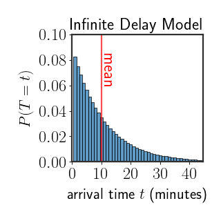
Amazingly, the only discrete, memoryless, distribution is the geometric distribution: \(\begin{equation} \forall\ t=1,2,\cdots \qquad\quad P\left(T=t\right)=\theta\cdot\left(1-\theta\right)^{t} \end{equation}\)where $\theta\in[0,1]$ is a parameter of the distribution that has to be defined in some manner. We know that a bus arrives approximately every 10 minutes, that is the mean of the distribution has to be equal to 10; we can use this to choose $\theta$. Luckily for us, the geometric distribution is a well known distribution and it’s mean is equal to: \(\begin{equation} \mathbb{E}[T]=\frac{1-\theta}\theta \end{equation}\) So, if we know that $\mathbb{E}[T]=M=10$, we can set $\theta=\frac{1}{M+1}$ to satisfy the constraint of the average arrival time. Here’s the corresponding distribution:
Modeling Finite Delays
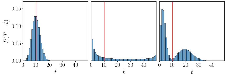
Okay, so a geometric distribution (which we will call the “infinite delay model” from now on) is much better than the deterministic model, but it doesn’t make sense that a bus could be “infinitely” delayed. As long as the bus’s route is sound and wasn’t canceled or something, the bus should probably arrive within the same day, if not earlier. This is another tidbit of information we can take into account when defining our model. In other words, we still believe that the variability between the delays is very large, but there is also a “maximal waiting time” which we will take into account.
So, how do we find a model that takes into account that the delays have to be finite? For the last two settings we had sound arguments which led us to a unique distribution of arrival times. This time however, there are numerous distributions that could fit our setting, the setting where the mean is known and the number of possible arrival times is finite. Here are three such possible distributions with a wait time of 50 minutes:
A Broader Look
If we take a step back for a moment, we can appreciate that what we’re looking for is more general than the issue of arrival times of busses. Abstracting the problem at hand reveals a much more fundamental question:
Given a set of constraints, is there a principled way to find a probabilistic model that will satisfy said constraints without assuming further information?
By principled we mean a single, unified, approach to choosing the distribution; no matter which constraints are given, we will know what needs to be done in order to find a distribution that satisfies them. Both the deterministic and geometric settings were definitely not solved in a principled manner: a different argument had to be made up for each specific case and were quite distinct from each other, predicated on our knowledge of esoteric properties of distributions.
Well, how about we find a single way to solve problems of this kind, one that we can always repeat and understand?
Maximum Entropy
To choose between a set of possibilities, we need a criterion which will tell us which distribution is “best”. This criterion is subjective, but important. Usually in mathematical modeling, distributions that do not insert any further bias are preferred - those that do not assume we have access to more information than we have observed. Simply put, we would usually prefer a model which is as “generic” as possible while still capturing quantities we care about.
This sounds reasonable, but what does it even mean for a distribution to be generic? Consider the following two distributions:
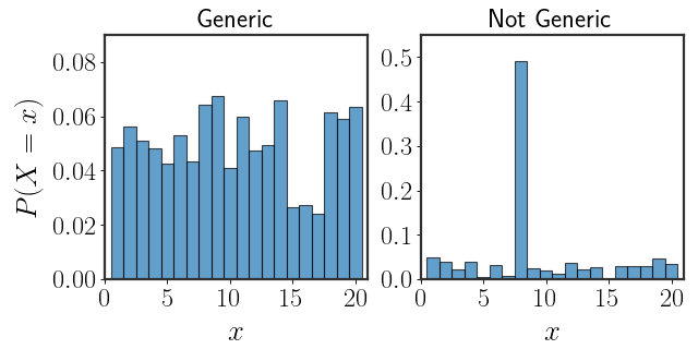
The distribution on the left spreads out the probability almost equally among all possible outcomes. Conversely, the one on the right assigns most of the probability to a single outcome. Which would you call more generic?
Well, the distribution on the right represents a very specific setting where one of the values is so much more probable than all of the other values. On the other hand, the distribution on the left is how we would describe a setting we know very little about. If we’ve only seen very few real-world samples, we would probably choose to model the empirical distribution with the more uniform distribution, since it assumes less. In particular, it doesn’t assume that one of the values is significantly more probable to occur.
Let’s try to build up a measure for the genericness of a distribution.
Enter Shannon
Looking at $P(X=x)$ for a specific value of $x$ already gives us a strong indication of whether a distribution is generic or not, right? If $P(x)$
There are many many ways to define $I(\cdot)$ so it’s behavior will match our abstract description. But, it would be nice if the function $I(\cdot)$ could also have the following properties:
- As we said, values with higher probabilities are more informative (less uninformative), so $I(x)$ should be monotonically decreasing with $P(x)$
- Since we are going to attempt to find distributions that maximize the genericness, it would help if $I(\cdot)$ were continuous in $P(x)$ (so we could differentiate the genericness with respect to the probabilities). In turn, we need $I(x)$ to be continuous in $P(x)$
- If $P(x)=1$, i.e. the outcome is certain, then $I(x)=0$, the lowest possible value
- If we observe two different outcomes, say $x_1$ and $x_2$, the uninformative-ness of one shouldn’t effect the uninformative-ness of the other. That is to say, the product of uninformative-ness of a couple values should be equal to their sum: \(\begin{equation} I(x_1\cdot x_2)=I(x_1)+I(x_2) \end{equation}\)
Under these criteria, finding a specific form is (perhaps suspiciously) simple. Properties 1 and 2 are easily met if $I(x)=f(\frac{1}{P(x)})$ and $f(\cdot)$ is a continuous, monotonically increasing function. Of these possible functions, the first that comes to mind that combines properties 3 and 4 is the logarithm
So, as long as our earlier requirements for un-informativeness make sense, the genericness of a distribution is given by: \(\begin{equation} \text{genericness}=-\sum_x P(x)\log P(x) \end{equation}\) Now, actually, this value has a much better name than “genericness”; it is the entropy of a distribution, usually denoted by: \(\begin{equation} H(X)=-\sum_x P(x)\log P(x) \end{equation}\)
Back to Our Busses - a Sanity Check
Before continuing on, let’s see whether maximizing the entropy really results in the distribution we’ve chosen for the deterministic model from earlier in this post. A simple sanity check to see that we are faithful to our earlier work.
For the deterministic model, the only unknown factor is when you arrive between the equally spaced busses. So, the distribution is over a finite set of values $T\in\left{1,\cdots,10\right}$, and that is the only thing we know about it. As mentioned before, the uniform distribution is the one with the highest entropy (in other words, is most generic) on a finite support. This is the same distribution as we saw before!
The fact that using the entropy is consistent with our earlier arguments is reassuring. But, how about the infinite delay model, the one with the geometric distribution? Well, for that we need to insert the fact that we know the mean of the distribution into this framework.
Adding Constraints
Back to the problem at hand. We have a set of constraints and want to find the most general distribution possible that still satisfies these constraints. So, what were our constraints?
- The distribution is discrete $T\in\left{1,\cdots,K\right}$ (let’s assume there are only finitely many values for now)
- The mean of the distribution is equal to $M$
Let’s rewrite the probabilities as: \(\begin{equation} p_t=P(T=t) \end{equation}\) This doesn’t change anything, but makes the next part a bit easier to write.
Basically, we want to solve the following maximization problem: \(\begin{equation}\label{eq:maximization} \begin{aligned} (p_1,\cdots,p_K)&=\arg\max_{\tilde{p}_1,\cdots,\tilde{p}_K} H(\tilde{p}_1,\cdots,\tilde{p}_K)\\ \text{subject to:}\quad & (I)\quad\sum_{t=1}^Kt\cdot \tilde{p}_t=M\\ & (II)\quad\forall t\quad \tilde{p}_t\ge 0\\ & (III)\quad \sum_{t=1}^K\tilde{p}_t=1 \end{aligned} \end{equation}\) This looks like a lot. Unpacking the constraints, we have: $(I)$ the mean is equal to $M$ (where it all started), $(II)$ all of the probabilities are larger than 0 and $(III)$ the probabilities sum up to 1. Again, it looks quite complicated, but actually constraints $(II)$ and $(III)$ just make sure that $p_1,\cdots, p_K$ is a proper distribution.
Enter Boltzmann
Honestly, solving the problem in equation \eqref{eq:maximization} doesn’t look easy. Instead of directly trying to do so, it will be better to try and get some intuition of what’s actually happening.
The Simplex
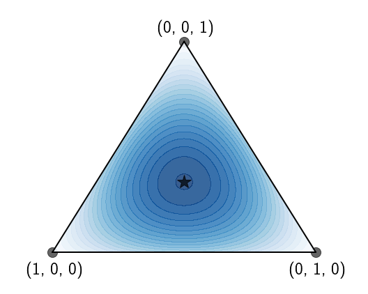
As we saw, constraints $(II)$ and $(III)$ just make sure that we’re maximizing over the set of proper distributions. But how what is this space of all proper distributions?
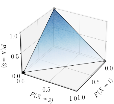
If a random variable can take a finite set of values (again, the thing we’re actually interested in) all possible distribution are inside what is called the simplex. The simplex is the set of all vectors of length $K$ whose elements are nonnegative and sum up to 1 - does that sound familiar?
Here’s a concrete but simple example. Forget about the distribution of busses for a second, let’s look at a random variable that can only take on 3 values, $X\in{1, 2, 3}$. All possible distributions over $X$ can be written as vectors of size 3: \(\begin{equation} \left(\begin{matrix}P(X=1)\\P(X=2)\\P(X=3)\end{matrix}\right)=\left(\begin{matrix}p_1\\p_2\\p_3\end{matrix}\right) \end{equation}\)
However, because the three elements $p_1,p_2,p_3$ have to sum up to 1, if we know $p_1$ and $p_2$ then $p_3$ is known and given by: \(\begin{equation} p_3=1-p_1-p_2 \end{equation}\) That way, we know for sure that $p_1+p_2+p_3=1$. So in fact, if $p_1$ and $p_2$ are known, $p_3$ can be deterministically set.
So, the set of all 3-dimensional distributions can actually be visualized in 2 dimensions, the simplex:
(As an aside, using the same reasoning any $D$-dimensional distribution can be described by a $(D-1)$ -dimensional vector.)
Entropy with Constraints
Visualizing the set of possible distributions in this manner allows us to easily overlay the entropy on top of the simplex:
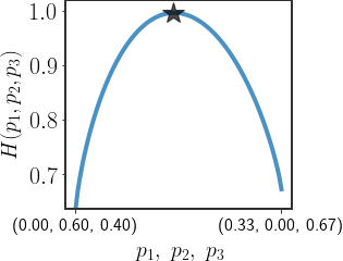
We started all of this by saying we want to constrain the mean of the distribution to be equal to $M$. We can now directly visualize this, focusing our search to a specific region on the simplex:
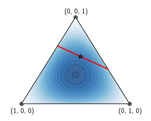
So, if we want to find the distribution that maximizes the entropy whose mean is equal to a specific value, all we have to do is find the maximal entropy in the region depicted by the constraint!
In fact, using this we can maximize the entropy under any constrain we want and with as many of them as we want, as long as there exists a distribution that satisfies all of the constraints. Different constraints will force us to search in different parts of the simplex, but in theory any constraint is valid.
Boltzmann Distributions
Okay, okay, so we have some basic intuition for what we’re trying to do. Now, how do we find the maximum entropy distribution mathematically?
For now, let’s restrict ourself constraints of the form
To find the maximum, we need to use Lagrange multipliers. Under their framework, we define the following function: \(\begin{equation} \mathcal{L}\left(p_1,\cdots,p_K,\lambda,\gamma\right)=\underbrace{H(X)}_{\text{entropy}}-\lambda\cdot\left(\sum_x p_xf(x)-F\right)-\gamma\cdot\left(\sum_x p_x-1\right) \end{equation}\) If you haven’t heard of Lagrange multipliers, all you need to know is that the stationary points of $\mathcal{L}(\cdot)$ will also be stationary points of our constrained problem. These stationary points will (after some math) give us the following form for the distribution: \(\begin{equation} P(X=x)=p_x=\frac{1}{Z}e^{\lambda f(x)}\qquad\quad Z=\sum_xe^{\lambda f(x)} \end{equation}\)
Click here to see the derivation
We need to find the stationary points of the function $\mathcal{L}(\cdot)$ with respect to $p_1,\cdots,p_K$ as well as $\lambda$ and $\gamma$. Notice that $\mathcal{L}(\cdot)$ is convex in all of these (the entropy is a convex function)! This is a good thing - we can just differentiate, equate to 0, and we will have found the maximum.
We’ll do just that: \(\begin{equation} \begin{aligned} \frac{\partial\mathcal{L}}{\partial p_x} = -\log p_x-\frac{p_x}{p_x} &-\lambda\cdot f(x)-\gamma\stackrel{!}{=}0\\ \Rightarrow \log p_x &= \lambda\cdot f(x)+\gamma+1\\ \Rightarrow p_x &= e^{\lambda f(x)}\cdot \Gamma \end{aligned} \end{equation}\) where, for simplicity, we have defined $\Gamma=\exp[\gamma + 1]$. So we have the general form of the distribution… all that’s left is to find what $\Gamma$ equals.
We can find the value of $\Gamma$ (by extension $\gamma$) by making sure that the distribution sums up to 1: \(\begin{equation} \begin{aligned} \sum_x p_x&=\Gamma\cdot\sum_x e^{\lambda f(x)}=1\\ \Rightarrow \frac{1}{\Gamma}=Z&= \sum_x e^{\lambda f(x)} \end{aligned} \end{equation}\)
This distribution is called the Boltzmann distribution and the normalization constant $Z$ is called the partition function (it is a function, just of $\lambda$ not of $x$)
The only problem is that we still have that pesky $\lambda$ stuck in there. We can find $\lambda$ by ensuring that our original constraint is satisfied: \(\begin{equation} \sum_x P(x)\cdot f(x)=F\ \ \Leftrightarrow \ \ \frac{1}{Z}\sum_x e^{\lambda f(x)}f(x)=F \end{equation}\) Unfortunately, analytically finding $\lambda$ in general is actually quite difficult; usually, numerical methods are used to find it.
One Last Sanity Check
A while ago we introduced a setting where the bus can be infinitely delayed and all we know is that the average wait time between busses is $M$ minutes. Our model in this setting was the geometric distribution with parameter $\theta=\frac{1}{M+1}$. Let’s try to make sure that this really is the distribution that maximizes the entropy.
Because our only constraint is the mean, we need to solve: \(\begin{equation} \begin{aligned} \frac{1}{Z}\sum_{t=1}^\infty e^{\lambda t}\cdot t &\stackrel{!}{=}M \\ \Leftrightarrow \sum_{t=1}^\infty e^{\lambda t}\cdot t&\stackrel{!}{=}M\cdot \sum_{t=1}^\infty e^{\lambda t} \end{aligned} \end{equation}\) Let’s break this problem into smaller parts and look at the following geometric series: \(\begin{equation} \sum_{t=1}^\infty \left(e^\lambda\right)^t \end{equation}\) This geometric series converges so long as $e^\lambda<1$. For now, let’s just assume that this actually happens. Then: \(\begin{equation} \sum_{t=1}^\infty \left(e^\lambda\right)^t = \frac{1}{1-e^\lambda} \end{equation}\)
We are one step closer. We now only need to find a $\lambda$ so that: \(\begin{equation} \sum_{t=1}^\infty e^{\lambda t}\cdot t\stackrel{!}{=}\frac{M}{1-e^\lambda} \end{equation}\) Now it’s time to take care of the left hand side of this equation. Notice that: \(\begin{equation} \sum_{t=1}^\infty e^{\lambda t}\cdot t=\sum_{t=1}^\infty \frac{d}{d\lambda}e^{\lambda t}=\frac{d}{d\lambda}\frac{1}{1-e^\lambda}=\frac{e^\lambda}{\left(1-e^\lambda\right)^2} \end{equation}\)
Plugging this in (after some algebra), gives the following value for $\lambda$:
\[\begin{equation} \lambda = \log\frac{M}{M+1} \end{equation}\]Click here if you want to see the algebra needed to get there
\[\begin{aligned} \frac{e^\lambda}{\left(1-e^\lambda\right)^2}&=\frac{M}{1-e^\lambda}\\ \Rightarrow \frac{e^\lambda}{1-e^\lambda}&=M\\ \Rightarrow\frac{1}{e^{-\lambda}-1}&=M\\ \Rightarrow e^{-\lambda} &=\frac{1}{M}+1\\ \Rightarrow \lambda &= \log(\frac{M}{M+1}) \end{aligned}\]Recall that we assumed that $e^\lambda < 1$ - let’s just quickly make sure that this is correct. Notice that $1+\frac1M > 1$, so $\log(1+\frac1M)>0$. So, $\lambda$ is negative, thus $e^\lambda=\frac{1}{e^{\vert\lambda\vert}}<1$ and everything is okay.
This doesn’t look like the geometric distribution yet, but let’s shift around some of the terms. Simplifying the smallest element of the distribution is always a good first step: \(\begin{equation} \begin{aligned} e^{\lambda t}&=\left(e^\lambda\right)^t=\left(\frac{M}{M+1}\right)^t \end{aligned} \end{equation}\) Plugging this into the partition function we get yet another geometric series (no wonder the distribution is called geometric): \(\begin{equation} Z=\sum_{t=1}^{\infty}\left(\frac{M}{M+1}\right)^t=\frac{1}{1-\frac{M}{M+1}}=M+1 \end{equation}\) Finally, finally, we substitute everything in to get: \(\begin{equation} P(T=t)=\left(1-\frac{M}{M+1}\right)\left(\frac{M}{M+1}\right)^t=\left(1-\frac{1}{M+1}\right)^t\cdot\frac{1}{M+1} \end{equation}\) which is exactly the definition of a geometric distribution with parameter $\theta=\frac{1}{M+1}$!
Back to Modeling Finite Delays
Unfortunately, there is no closed form solution to the maximization problem in equation \eqref{eq:maximization}. So, if we want to model finite delays in our bus arrival distribution, we have to solve the maximization problem numerically, except for a few settings. These specific cases will give us at least some intuition for the general behavior of the solution.
Let’s refresh our memory. We are trying to find a distribution over a random variable $T\in\left{1,\cdots, T_{\text{max}}\right}$ whose mean is equal to $M$. In the tardy bus setting, $M=10$ and $T_{\text{max}}$ is the largest number of minutes conceivable for the bus to be delayed. For instance, if there is no way that the bus can be more than an hour late, we can set $T_{\text{max}}=60$.
From our earlier explorations, we saw that the max-entropy distribution under these constraints will be the Boltzmann distribution: \(\begin{equation} P(T=t)=\frac{1}{Z} e^{\lambda t} \end{equation}\) where: \(\begin{equation}\label{eq:mean-maxent} \frac{1}{Z}\sum_{t=1}^{T_{\text{max}}} t\cdot e^{\lambda t}=M \end{equation}\) Of course, a solution only exists when $1\le M\le T_{\text{max}}$.
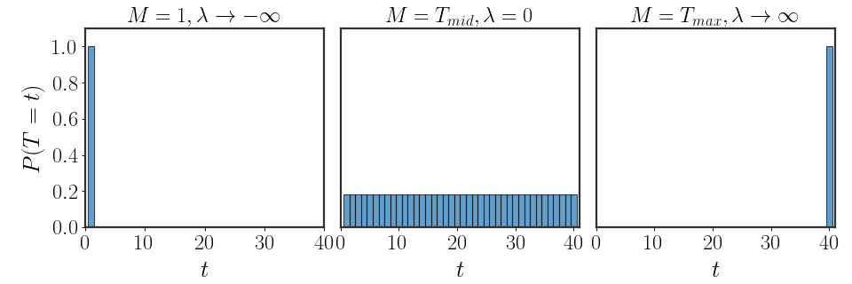
Both Sides of the Extreme
Before using numerical methods, notice that when $M=1$ or $M=T_{\text{max}}$, we can find an analytical solution. In both cases, the only distribution that satisfies equation \eqref{eq:mean-maxent} is the indicator: \(\begin{equation} \begin{aligned} M=1:&\quad P(T=t)=\begin{cases}0&t\neq1\\1&t=1\end{cases}=\bf{1}_{\left[t=0\right]}\\ M=T_{\text{max}}:&\quad P(T=t)=\begin{cases}0&t\neq T_{\text{max}}\\1&t=T_{\text{max}}\end{cases}=\bf{1}_{\left[t=T_\text{max}\right]} \end{aligned} \end{equation}\)
What are the values of $\lambda$ that give us such behaviors? Well, when $M=1$, we can rewrite our distribution as: \(\begin{equation} P(T=t)=\frac{e^{\lambda t}}{\sum_{\tau=1}^{T_{\text{max}}} e^{\lambda \tau}}=\frac{e^{\lambda t}}{e^{1\cdot\lambda}\cdot\left(1+\sum_{\tau=2}^{T_\text{max}e^{\lambda(\tau-1)}}\right)}=\frac{e^{\lambda(t-1)}}{1+\sum_{\tau=2}^{T_\text{max}e^{\lambda(\tau-1)}}} \end{equation}\) Writing the distribution in this manner is quite revealing. Let’s see what happens when $t=1$: \(\begin{equation} P(T=1)=\frac{e^{\lambda\cdot0}}{1+\sum_{\tau=2}^{T_\text{max}e^{\lambda(\tau-1)}}}=\frac{1}{1+\sum_{\tau=2}^{T_\text{max}e^{\lambda(\tau-1)}}} \end{equation}\) For any other value, the distribution will be proportional to $e^{\lambda(t-1)}$. Now, if we can find a value of $\lambda$ for which $e^{\lambda(t-1)}=0$ for all $t>1$, then we will have found our solution. So, when does this happen?
Well, only at the limit $\lambda\rightarrow -\infty$. At this limit, we get the correct distribution. Using exactly the same arguments, when $M=T_\text{max}$ it can be shown that $\lambda\rightarrow\infty$.
Uniform, Again?!
Actually, there is an additional situation with an analytical solution. If $M=\frac{1+\cdots+T_{\text{max}}}{T_{\text{max}}}=T_\text{mid}$, then equation \eqref{eq:mean-maxent}: \(\begin{equation} \sum_{t=1}^{T_\text{max}}\frac{e^{\lambda t}}{Z}\cdot t=\frac{1}{T_\text{max}}\sum_{t=1}^{T_\text{max}}t=T_\text{mid} \end{equation}\) Of course, this can only happen when $P(T=t)$ is the same for all values of $t$ - the uniform distribution (again)! What does $\lambda$ equal in this case? Well, the only option is that $\lambda=0$; that’s the only way that $P(T=t)$ will be the same for all values of $t$.
Somewhere Inbetween
Let’s put all of the values of $\lambda$ that we’ve found so far next to each other:
\[\begin{aligned} M=1\ :&\qquad \lambda\rightarrow-\infty\\ M=T_\text{mid}\ :&\qquad \lambda=0\\ M=T_\text{max}\ :&\qquad \lambda\rightarrow\infty\\ \end{aligned}\]See how there seems to be an ordering according to $\lambda$? From the lower extreme case ($M=1$), through the middling solution of the uniform distribution, and to the other side ($M=T_\text{max}$). Every solution between any of these values will have some aspect of their neighbors’:
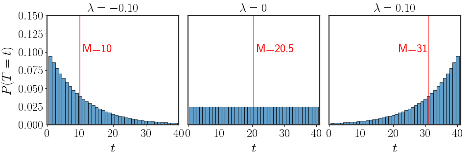
Using the analytical outcomes, we can expect that
Numerically Finding Solutions
Unfortunately, as mentioned, finding an analytical form for the max-entropy is difficult or completely impossible. Instead, we use numerical methods to maximize the entropy under our constraints.
One key feature of max-entropy is that it is relatively easy to find solutions. In the first place, the entropy is a convex function. So, as long as the constraint defines a convex set
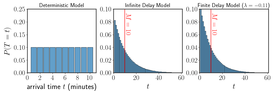
Honestly, the solution to the problem as we set out to solve might not be totally interesting. Here are all of our models together (with numerical estimation):
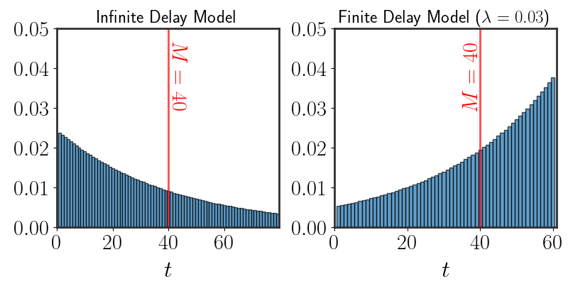
Playing around with the average time we expect the bus to arrive reveals more interesting behavior:
Wrapping Up
Whew, that was a lot. Quite a ride.
Starting from a naive question, we went through a lot of trouble to find the answer. The framework we derived in this post is aptly called the max-entropy principle, and was first introduced by Jayne back in 1957. But, most of the math used in this post actually originates from even earlier sources.
In the late 19th century, Boltzmann (and later Gibbs) revolutionized thermodynamics and gave us a much deeper understanding of the field by showing how its fundamental equations could be derived using probabilistic arguments. It turns out, as we just explored in this post, that the mathematical tools they developed are relevant for much more than molecules bumping into each other. The concept of entropy started out as an abstract property of a thermodynamic system, later redefined by Boltzmann and Gibbs using their statistical physics framework, and eventually generalized by Shannon to a concept relevant to all of statistical inference.
The same principles originally introduced for statistical physics are now used widely in machine learning and statistics. Since the maximum entropy principle is simply a way to find distributions that are generic while retaining known information, it is a method used for scientific discovery and modeling in a range of fields.
Hopefully, even though a bit of math was involved, you now know how to model distributions under different constraints.
Outro
It is now 25 minutes later. The bus arrived, a bit late but not too bad, and you got to the exam just in time! You found a general solution for the problem you originally posed. It took the whole bus ride, you originally wanted to go over some last-minute details for the exam, but maybe this is okay as well?
May all of your busses arrive on time!