More on Kernel Regression
Having defined kernels, this post delves into how such kernels can be used in the context of linear regression. This results in an extremely powerful model, but also adds computational problems when confronted with vast amounts of data.
In the previous post we defined kernels, showed how they can be constructed, and even showed how to use them together with ridge regression. In this post, we’re going to take a closer look at kernel ridge regression and the implications of using kernels instead of basis functions.
Last time, we basically showed that if we assume a zero-mean, diagonal Gaussian prior on the parameters $\theta\sim\mathcal{N}(0,I\lambda)$ , then the MMSE solution for linear regression is given by:
\[\begin{equation} \hat{\theta} = \left(\frac{\sigma^{2}}{\lambda}I+H^{T}H\right)^{-1}H^{T}y =H^{T}\left(\frac{\sigma^{2}}{\lambda}I+HH^{T}\right)^{-1}y \end{equation}\]To predict the function at a new point, we only need to calculate:
\[\begin{align} y_{\hat{\theta}}\left(x\right) & =h^{T}\left(x\right)H^{T}\left(\frac{\sigma^{2}}{\lambda}I+HH^{T}\right)^{-1}y\\ & =y^{T}\left(\frac{\sigma^{2}}{\lambda}I+HH^{T}\right)^{-1}Hh\left(x\right) \end{align}\]If we assume that the inner product is given by some kernel, i.e. $h^{T}\left(x\right)h\left(y\right)=k\left(x,y\right)$ , and that $K$ is the Gram matrix of the kernel on the data points $\{x_i \}_{i=1}^{N}$ such that $K_{ij}=k\left(x_{i},x_{j}\right)$, then:
\[\begin{align} y_{\hat{\theta}}\left(x\right) & =y^{T}\left(\frac{\sigma^{2}}{\lambda}I+K\right)^{-1}\left(\begin{matrix}h^{T}\left(x_{1}\right)h\left(x\right)\\ \vdots\\ h^{T}\left(x_{N}\right)h\left(x\right) \end{matrix}\right) \\ & =y^{T}\left(\frac{\sigma^{2}}{\lambda}I+K\right)^{-1}\left(\begin{matrix}k\left(x,x_{1}\right)\\ \vdots\\ k\left(x,x_{N}\right) \end{matrix}\right) \\ & =\sum_{i=1}^{N}\left[y^{T}\left(\frac{\sigma^{2}}{\lambda}I+K\right)^{-1}\right]_{i}k\left(x,x_{i}\right) \\ & \stackrel{\Delta}{=}\sum_{i=1}^{N}\alpha_{i}\cdot k\left(x,x_{i}\right)\label{eq:dual-form} \end{align}\]where $N$ is the number of data points we have in the data set. Notice that this problem looks exactly like the regular linear regression, only with new basis functions ($N$ of them).
This is called the solution to the dual problem. In fact, we’ve already seen how to find this solution, when we derived an equivalent expression for Bayesian linear regression. The main point is that whenever we have the inner product over features $HH^T$, we instead use our trusty kernel.
No Sample Noise
Notice that if we take $\sigma^{2}=0$, the solution becomes:
\[\begin{equation} f\left(x\right)=h^{T}\left(x\right)H^{T}K^{-1}y \end{equation}\]in which case we have to assume that the Gram matrix is invertible for there to be a solution. Since the Gram matrix is PSD (by definition), the only way that it can be invertible is if it is PD as well, i.e. if the kernel $k\left(\cdot,\cdot\right)$ is a PD kernel.
Anyway, let’s look at the prediction of the train points, and see what we get. The prediction in this case will be given by ($\hat{y}$ below is the vector of predictions for all of the training data points $x_{i}$):
\[\begin{equation} \hat{y}=HH^{T}K^{-1}y=Iy=y \end{equation}\]and in fact our training error will be 0! What does this tell us?
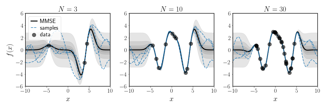
If the kernel $k\left(\cdot,\cdot\right)$ is PD, then it can fit any function. In particular, for any finite set of points $\{ x_{i}\}_{i=1}^{N}$, the set of basis functions $\{ k\left(x,x_{i}\right)\}_{i=1}^{N}$ spans all possible functions that pass through the points $\{ \left(x_{i},y\left(x_{i}\right)\right)\}_{i=1}^{N}$.
Example: RBF Kernel
Showing it explicitly is kind of a pain, but the Gaussian kernel is a PD kernel:
\[\begin{equation} k\left(x,y\right)=e^{-\beta\vert x-y\vert ^{2}} \end{equation}\]Let’s take a look at the basis functions this kernel induces in the dual form (as in equation \eqref{eq:dual-form}). For any set of training points $\{ x_{i}\}_{i=1}^{N}$, using the Gaussian kernel is like fitting the following linear regression problem:
\[\begin{align} f\left(x\right) & =\sum_{i=1}^{N}\alpha_{i}k\left(x,x_{i}\right)\\ & =\sum_{i=1}^{N}\alpha_{i}e^{-\beta\vert x-x_{i}\vert ^{2}}\\ & =\sum_{i=1}^{N}\alpha_{i}\varphi_{x_{i}}\left(x\right) \end{align}\]where $\varphi_{\mu}\left(\cdot\right)$ is the Gaussian basis function centered around the point $\mu$. So, in fact, using kernel ridge regression with a Gaussian kernel is the same as using $N$ Gaussian basis functions, centered around each of the data points. This (hopefully) makes sense - if we have a Gaussian around each data point $x_{i}$, then finding the weights of each basis function so that they pass through the points $y\left(x_{i}\right)$ sounds easy.
Choosing Kernels, Not Basis Functions
Up until now, we have been choosing the basis functions we want to use in order to define the linear regression problem. This view of the problem was helpful when we defined the basis functions explicitly, but now that we moved to kernel regression, it is less informative. Now, instead of choosing basis functions, we choose a kernel which (implicitly) defines an inner product between sets of basis functions. But how can we choose the kernels in an informative manner?
When choosing kernels, instead of basis functions, we want to choose the expected behavior of the regressed function - how smooth it looks, how fast it alternates between values, if it’s periodic, etc. In this sense, we change the characteristics of the functions through the kernels. In the dual form (as in equation \eqref{eq:dual-form}), the prior we have over the parameters $\alpha$ is:
\[\begin{equation} \alpha\sim\mathcal{N}\left(0,K^{-1}\right) \end{equation}\]where $K$ is the Gram matrix of the training points using the kernel. As we can see, the choice of kernel is directly reflected in our prior. In particular, the kernel controls the structure of the covariance between data points, so it makes sense to choose the kernel to reflect a sense of similarity between points.
Example: Changing the Bandwidth of the RBF Kernel
Let’s look at the Gaussian kernel, again.
The parameter $\beta$ is called the bandwidth of the kernel, and defines how quickly we expect changes in the data. Specifically, let’s look at the two extremes $\beta\rightarrow\infty$ and $\beta\rightarrow0$:
\[\begin{align} \forall x\neq y\quad e^{-\beta\vert x-y\vert ^{2}} & \stackrel{\beta\rightarrow\infty}{=}e^{-\infty}=0\\ e^{-\beta\vert x-y\vert ^{2}} & \stackrel{\beta\rightarrow0}{=}e^{0}=1 \end{align}\]But what does this tell us?
Specifically, when $\beta\rightarrow0$, then the estimate of the function becomes:
\[\begin{equation} f_{0}\left(x\right)=\sum_{i=1}^{N}\alpha_{i} \end{equation}\]so we are trying to fit a straight line. This means that the kernel we chose expects all values of the function to be the same - given 1 point, we know how all others should behave. We can call this function “infinitely smooth”, in the sense that the fitted line will have no derivative at all. Alternatively we could the function “unragged”, but that sounds a bit weird.
On the other hand, when $\beta\rightarrow\infty$ the Gram matrix will be:
\[\begin{equation} K_{\infty}=I \end{equation}\]so the prior over the parameters will be the standard normal distribution, so the $x_{i}$-th point doesn’t really care about the value of the function at the $x_{j}$-th point. The MMSE solution in this case is:
\[\begin{equation} f_{\infty}\left(x\right)=\begin{cases} 0 & x\not\in\left\{ x_{i}\right\} _{i=1}^{N}\\ y_{i} & x=x_{i} \end{cases} \end{equation}\]This is a kind of useless function as well, since it will only know the values of the function at the points from the training data. The functions we fit with this function can be “infinitely ragged”, in this sense.
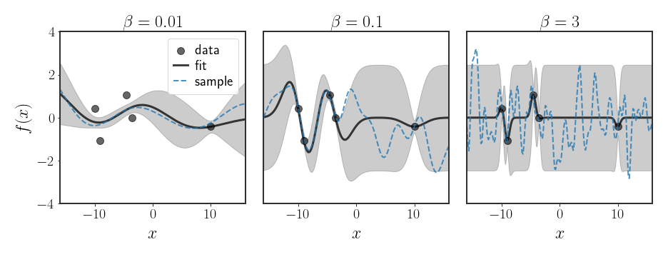
As we can see, the bandwidth parameter $\beta$ controls “how ragged” we expect the function to be. This sentiment is mirrored in the figure below, where it is really clear that the large $\beta$ value pulls the functions towards more wiggly functions, while the really low value pushes the learned function into a really stretched out curve.
Numerical Complexity
Let’s look at the two versions of the MMSE solution again. Recall the matrix $H$ is a $p\times N$ matrix, where $p$ is the number of basis functions and $N$ is the number of points in the training data set. For the primal space we need to invert the matrix $H^{T}H+I\beta$ where $\beta$ is some number, which is a $p\times p$ matrix. In the dual formulation, we need to invert the matrix $HH^{T}+I\beta$ which is an $N\times N$ matrix. Typically, when we use kernels, we want to embed the data points $x_{i}$ into a much higher-dimensional space, so that $p\gg1$. Clearly, using the original linear regression solution is not practical (recall, for RBF kernels we have an infinite number of dimensions in the feature space).
Okay… so if we want to use (expressive) feature spaces, we should usually use the dual formulation. Right, so while in the “classical” sense, inverting an $N\times N$ matrix is probably fine (since the number of points isn’t gigantic), in modern machine learning we use millions (if not billions) of data points in order to learn our estimators. Meanwhile, inverting a $1000\times1000$ matrix is already pretty difficult, never mind a $10^{6}\times10^{6}$ matrix which we probably can’t even store in memory
Using Less Points
Since we saw that the problem with the dual solution is that fact that we need to invert a matrix that is $N\times N$, the simplest solution is simply to choose some number $M<N$ and use $M$ train points instead of all of the $N$ data points, where $M$ is sub-sampled from the original points in some manner
The problem then becomes: how do we choose which points to use?
Subset of Data
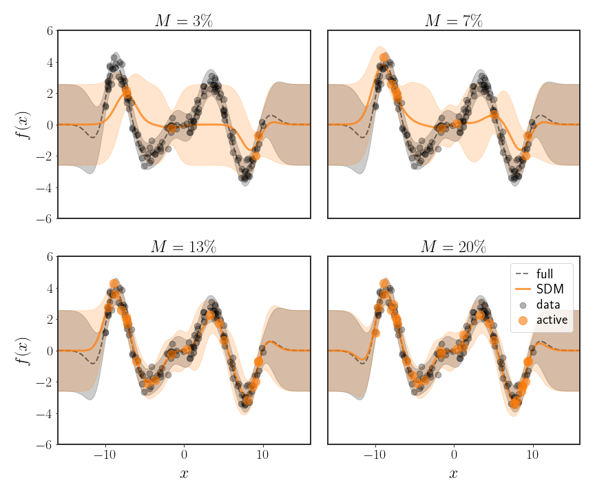
Simply choosing a subset of the data and throwing out all of the rest is sometimes called the subset of data method (SDM). The easiest way to do this is to randomly choose the subset of size $M$ from all of the points, but this has some obvious drawbacks. This protocol is the one used in the figure 3 below, for different amounts of data that are kept. As you can see, while using 3% of the data is not very useful, we can still achieve pretty good results with 10% of the data (at least in this example). Because of the $O(N^{3})$ complexity of inverting a matrix, this means that we can save something like 3 orders of magnitude of computation (1000 times faster) with these 10% of samples - that’s pretty good!
Subset of Regressors
Recall that the kernel regression problem we saw is equivalent to:
\[\begin{equation} f\left(x\right)=\sum_{i=1}^{N}\alpha_{i}k\left(x_{i},x\right) \end{equation}\]with the prior $\alpha\sim\mathcal{N}\left(0,K^{-1}\right)$, where $K$ is the Gram matrix of the kernel $k\left(\cdot,\cdot\right)$ on the $N$ data points $\{ x_{i}\} _{i=1}^{N}$. However, if we use $M<N$ data points instead of the full data set, we can instead approximate the problem using:
\[\begin{equation} \tilde{f}\left(x\right)=\sum_{i=1}^{M}\tilde{\alpha}_{i}k\left(x_{i},x\right) \end{equation}\]where $\tilde{\alpha}\sim\mathcal{N}\left(0,K_{mm}^{-1}\right)$, such that $K_{mm}\in\mathbb{R}^{M\times M}$ is the Gram matrix on the subset of $M$ points. In practice, this means that we will attempt to use standard Bayesian linear regression with basis functions corresponding to the kernels centered around the subset of $M$ points (also called the active set).
Assume, without loss of generality, that the first $M$ points are those that were chosen and define:
\[\begin{equation} H=\left(\begin{matrix}-k^{T}\left(x_{1}\right)-\\ \vdots\\ -k^{T}\left(x_{N}\right)- \end{matrix}\right)\in\mathbb{R}^{N\times M} \end{equation}\]as our basis functions, where $k\left(\tilde{x}\right)=\left(k\left(x_{1},\tilde{x}\right),\cdots,k\left(x_{M},\tilde{x}\right)\right)^{T}\in\mathbb{R}^{N}$. The problem we are trying to fit for all $N$ data points can now be rewritten as:
\[\begin{equation} y=H\tilde{\alpha}+\eta\qquad\tilde{\alpha}\sim\mathcal{N}\left(0,K_{mm}^{-1}\right) \end{equation}\]which is just the definition of regular linear regression. Using this notation, the posterior will be given by:
\[\begin{equation} \alpha\vert \mathcal{D}_{M}\sim\mathcal{N}\left(\left(H^{T}H+\sigma^{2}K_{mm}\right)^{-1}H^{T}y,\;\left(\frac{1}{\sigma^{2}}H^{T}H+K_{mm}\right)^{-1}\right) \end{equation}\]and the MMSE solution will be:
\[\begin{equation} \tilde{f}\left(x\right)=k_{m}^{T}\left(x\right)\left(H^{T}H+\sigma^{2}K_{mm}\right)^{-1}H^{T}y \end{equation}\]where:
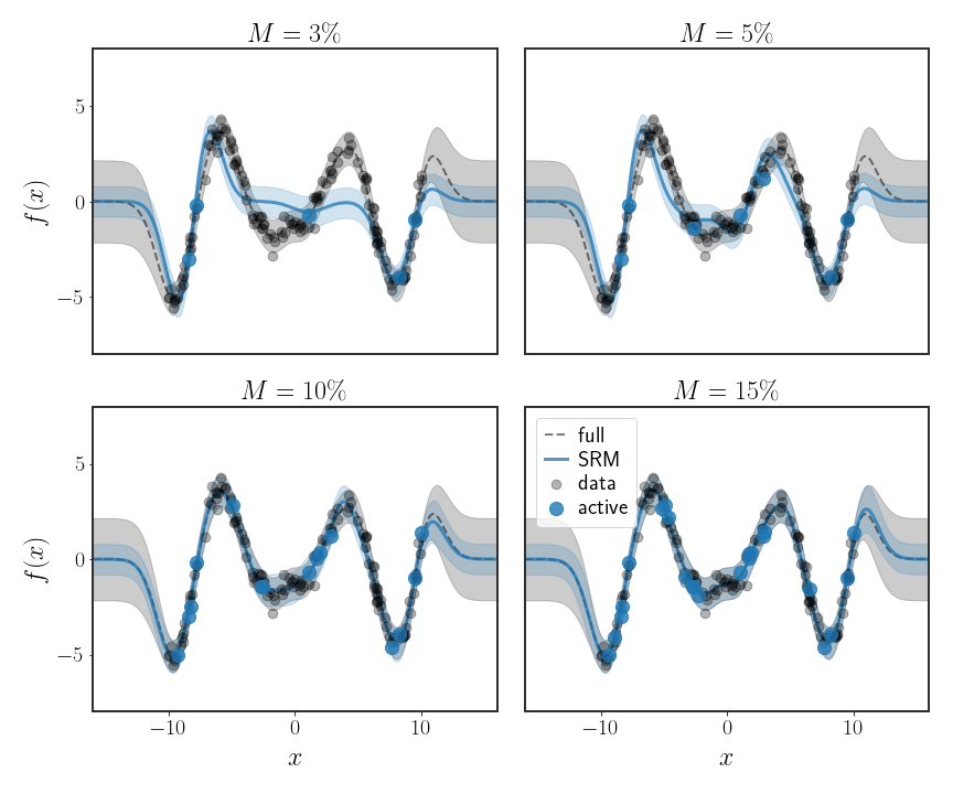
\[k_{m}\left(\tilde{x}\right)=\left(k\left(x_{1},\tilde{x}\right),\cdots,k\left(x_{M},\tilde{x}\right)\right)^{T}\in\mathbb{R}^{M}\]As you can see in the figure below, the MMSE prediction is much more accurate with fewer points than the subset of data method we saw before.
This is better than what we had before, but has a major drawback. Consider the variance of our prediction for a given data point:
\[\begin{equation} \text{var}\left[\tilde{f}\left(x\right)\right]=\sigma^{2}+k_{m}^{T}\left(x\right)\left(\frac{1}{\sigma^{2}}H^{T}H+K_{mm}\right)^{-1} k_{m}\left(x\right) \end{equation}\]Specifically, if the kernel $k\left(x,\tilde{x}\right)$ we are using decays the further $x$ is from $\tilde{x}$, then our predicted variance will decay faster than it should; this is really clear in all of the examples in figure 3, below -10 and above 10. This is obviously a problem that goes against the core Bayesian philosophy that we should know how uncertain we are about our predictions. To mitigate this affect, another option is to let the predicted value be given by:
\[\tilde{f}(x\_*)=\sum\_{i=1}^{M}\tilde{\alpha}\_{i}k\left(x\_{i},x\_{*}\right)+\alpha\_{*}k\left(x\_{*},x\_{*}\right)\]which can also be solved. Adding the additional $\alpha_{*}$ allows us to fix the predictive variance of the model (but we won’t get into that here).
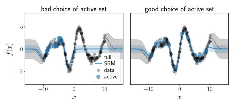
At any rate, now when we fit the parameters $\alpha$, we will take into account all data points, not just a subset of them (even though the problem is defined only on a subset). However, this method is still very sensitive to the choice of the subset chosen to represent all data points, as can be seen in the following figure:
Using Less Features
The whole point of using kernel regression was that we are suddenly able to use very expressive basis functions, without the cost of inverting the posterior covariance, which will have as many dimensions as there are basis functions. But, in the process, we became reliant on inverting an $N\times N$ matrix, which is infeasible when there are many data points. In the previous section we showed that we don’t really need to use all data points in order to fit our kernel machine, but can we instead use less features
Approximating Kernels
By Mercer’s theorem, if $k:\mathcal{X}\times\mathcal{X}\rightarrow\mathbb{R}$ is a valid kernel, then there exists a basis function $\varphi:\mathcal{X}\rightarrow\mathcal{V}$ such that:
\[\begin{equation} k\left(x,y\right)=\left\langle \varphi\left(x\right),\varphi\left(y\right)\right\rangle _{\mathcal{V}} \end{equation}\]where $\mathcal{V}$ is some vector space and $\left\langle \cdot,\cdot\right\rangle _{\mathcal{V}}$ is the inner product associated with $\mathcal{V}$. If this is the case, then perhaps there exists some map $z:\mathcal{X}\rightarrow\mathbb{R}^{q}$ such that:
\[\begin{equation} k\left(x,y\right)=\left\langle \varphi\left(x\right),\varphi\left(y\right)\right\rangle _{\mathcal{V}}\approx z^{T}\left(x\right)z\left(y\right) \end{equation}\]If such a map exists, then we can return to the primal form and use the basis functions defined by $z\left(\cdot\right)$ in order to perform standard Bayesian linear regression.
An example of such an approximation can be found through random Fourier features (RFF). In RFF, the basis functions are chosen so that they approximate the Fourier transform of the kernel as best as possible. Specifically, instead of using an infinite number of Fourier coefficients, a finite number is chosen which best represent the Fourier transform of the kernel. This trick can easily for any stationary kernel
Approximating the RBF kernel
The following was formalized in the article Random Features for Large-Scale Kernel Machines by Rahimi and Recht from 2007, which I highly recommend you to read.
Let’s look at a particular example. Suppose $\omega\sim\mathcal{N}\left(0,I\right)$ and define:
\[\begin{equation} \varphi_{\omega}:x\mapsto e^{i\omega^{T}x} \end{equation}\]where $i$ is the imaginary unit. In the complex plane, our usual transpose needs to be switched for the conjugate (because we’re using complex numbers), but otherwise everything is the same. Notice that: \(\begin{align} \mathbb{E}_{\omega}\left[\varphi_{\omega}^{*}\left(x\right)\varphi_{\omega}\left(y\right)\right] & =\mathbb{E}_{\omega}\left[e^{i\omega^{T}x}e^{-i\omega^{T}y}\right]\nonumber \\ & =\mathbb{E}_{\omega}\left[e^{i\omega^{T}\left(x-y\right)}\right]\nonumber \\ & =\intop p\left(\omega\right)e^{i\omega^{T}\left(x-y\right)}d\omega\nonumber \\ & \propto\intop e^{-\frac{1}{2}\vert \omega\vert ^{2}}e^{i\omega^{T}\left(x-y\right)}d\omega\nonumber \\ & =\intop\exp\left[-\frac{1}{2}\left(\vert \omega\vert ^{2}-2i\omega^{T}\left(x-y\right)\right)\right]d\omega\nonumber \\ & =\intop\exp\left[-\frac{1}{2}\left(\vert \omega\vert ^{2}-2i\omega^{T}\left(x-y\right)-\left(x-y\right)^{T}\left(x-y\right)\right)-\frac{1}{2}\left(x-y\right)^{T}\left(x-y\right)\right]d\omega\nonumber \\ & =e^{-\frac{1}{2}\vert x-y\vert ^{2}}\intop\underbrace{\exp\left[-\frac{1}{2}\vert \omega-i\left(x-y\right)\vert ^{2}\right]}_{\text{Gaussian integral}}d\omega\nonumber \\ & \propto e^{-\frac{1}{2}\vert x-y\vert ^{2}} \end{align}\)
Amazingly, this very simple, random, mapping $\varphi_{\omega}\left(\cdot\right)$ approximates the RBF kernel!
Let’s see how we can use this in practice. Suppose we sample $R$ i.i.d. values for $\omega$ from $\mathcal{N}\left(0,I\right)$, then: \(\begin{align} k\left(x,y\right) & =Ce^{-\frac{1}{2}\vert x-y\vert ^{2}}\\ & \overset{\star}{=}\intop\mathcal{N}\left(\omega\,\vert \,0,I\right)e^{i\omega^{T}\left(x-y\right)}d\omega\\ & =\mathbb{E}_{\omega}\left[e^{i\omega^{T}\left(x-y\right)}\right]\\ & \stackrel{\left(*\right)}{\approx}\frac{1}{R}\sum_{j=1}^{R}e^{i\omega_{j}^{T}\left(x-y\right)}\\ & \stackrel{}{=}\left(\begin{matrix}\frac{1}{\sqrt{R}}\exp\left(i\omega_{1}^{T}x\right)\\ \vdots\\ \frac{1}{\sqrt{R}}\exp\left(i\omega_{R}^{T}x\right) \end{matrix}\right)^{T}\left(\begin{matrix}\frac{1}{\sqrt{R}}\exp\left(i\omega_{1}^{T}y\right)\\ \vdots\\ \frac{1}{\sqrt{R}}\exp\left(i\omega_{R}^{T}y\right) \end{matrix}\right)\\ & \stackrel{\Delta}{=} h^{T}\left(x\right)h\left(y\right) \end{align}\)
where the step with the $\star$ is going back through the calculations we did before. We now see that the random mapping $h:\mathbb{R}^{d}\to\mathbb{R}^{R}$ approximates the RBF kernel using a finite number of basis functions, even though the RBF kernel uses an infinite number of basis functions. This is pretty cool - a random mapping behaves similarly to a pretty powerful kernel.
At the moment, our approximating basis functions are complex, even though our kernel is not. Looking at the step with the $\left(*\right)$, the term on the right hand side is complex while the one on the left hand side is not. Clearly, since they are (approximately) equal, we can remove the complex part. Using Euler’s formula, this is simple:
\[\begin{equation} e^{i\omega^{T}\left(x-y\right)}=\cos\left(\omega^{T}\left(x-y\right)\right)+\cancel{i\sin\left(\omega^{T}\left(x-y\right)\right)} \end{equation}\]Now, using some trigonometry:
\[\begin{equation} \cos\left(\omega^{T}x-\omega^{T}y\right)=\cos\left(\omega^{T}x\right)\cos\left(\omega^{T}y\right)+\sin\left(\omega^{T}x\right)\sin\left(\omega^{T}y\right) \end{equation}\]So, we can actually rewrite the basis functions as:
\(\begin{equation} h\left(x\right)=\frac{1}{\sqrt{R}}\left(\begin{matrix}\cos\left(\omega_{1}^{T}x\right)\\ \sin\left(\omega_{1}^{T}x\right)\\ \vdots\\ \cos\left(\omega_{R}^{T}x\right)\\ \sin\left(\omega_{R}^{T}x\right) \end{matrix}\right) \end{equation}\) where (again) $\omega_{i}\sim\mathcal{N}\left(0,I\right)$.
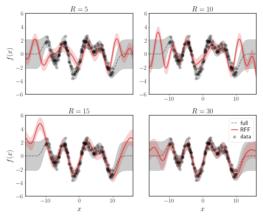
In practice, the RFF approximations are pretty efficient, where typically only $O\left(\sqrt{N}\right)$ random features are needed (where $N$ is the number of points) to get a very good approximation. For very large data sets, this becomes a very significant factor - for instance, with $N=10^{6}$ points, we would instead need $R=10^{3}$ features to guarantee a very good fit, which is doable. In practice, we can also use less random features and still get a suitable approximation.
An example use of RFF can be seen in the following figure:
Discussion
This was a long post. However, you now hopefully have a better understanding of kernel ridge regression, challenges with this regression, and even ways to get around said challenges.
One thing that remains kind of dodgy is that we never explicitly defined a prior over our infinite number of parameters. In fact, is a distribution on an infinite number of parameters even possible? The next post delves into this exact conundrum. We will show that yes, it’s possible to define a distribution on the infinite number of parameters, and it allows us to nicely consider the functional form of the regression.