Evidence Function
The evidence function (or marginal likielihood) is one of the cornerstones of Bayesian machine learning. This post shows the construction of the evidence and how it can be used in the context of Bayesian linear regression.
In the previous posts, we defined the problem of (Bayesian) linear regression and found the MLE and posterior for the linear regression parameters. Throughout, we kind of assumed that the basis functions and prior were somehow chosen ahead of time, and didn’t really talk about how to choose which basis functions to use. This is the focus of the current post.
As we have previously discussed, there are many possible basis functions $h\left(\cdot\right)$ we can use to fit the linear regression model, and it is not always so simple to determine which set of basis functions is the correct one to use. On one hand, if we use a very expressive set of basis functions (or a very large one) then the model will easily fit the training data but will probably give very inaccurate predictions for unseen data points. On the other hand, if we use a model that is too simplistic, then we will end up missing all of the data points.
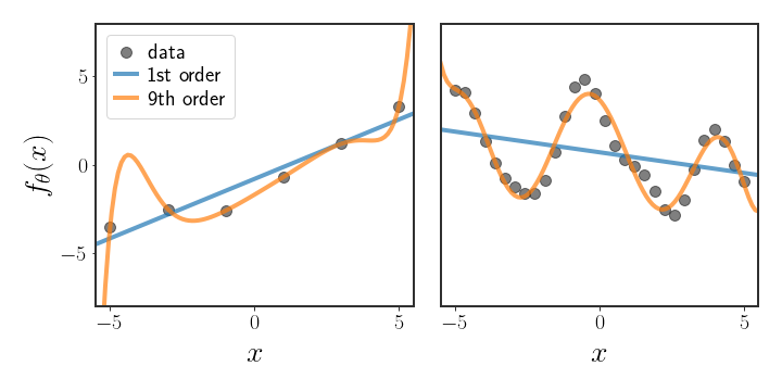
This is exactly the dilemma represented in figure 1; on the left, it is fairly obvious that the straight line should be chosen, although the 9th order polynomial fits the data better. The graph on the right shows exactly the opposite - the 9th order polynomial intuitively looks like it explains the data better than the linear function. However, in both cases the 9th order polynomial has much higher likelihood. So, how can we choose which of the basis functions is a better fit for the data?
The evidence function
The way it is written at the moment may be a bit confusing. Up until now (and from now on, as well), we wrote the prior as $p\left(\theta\right)$ , but suddenly we’re adding the conditioning on $\Psi$ - why? When we define a prior, we usually have to choose a distribution for the prior. Often, this distribution has (hyper)parameters that define it; for instance, if the prior is a Gaussian, then the parameters are the specific $\mu_{0}$ and $\Sigma_{0}$ we chose. In our new notation $\Psi=\{ \mu_{0},\Sigma_{0}\}$ , and we want to compare between different possible $\Psi$ s.
Example: Simple Bayesian linear regression
As an example, suppose we assume that:
\[\begin{align} y & =\theta x \end{align}\]Furthermore, we assume that we have two priors on $\theta$ given by:
\[\begin{align} \theta & \sim\mathcal{N}\left(\mu_{1},\Sigma_{1}\right)\\ \tilde{\theta} & \sim\mathcal{N}\left(\mu_{2},\Sigma_{2}\right) \end{align}\]In other words, we have two competing priors, from which we want to choose only one. We can then calculate:
\[\begin{equation} p\left(y\mid \mu_{i},\Sigma_{i}\right)=\intop p\left(y\mid \theta\right)p\left(\theta\mid \mu_{i},\Sigma_{i}\right)d\theta \end{equation}\]for $i\in\{ 1,2\}$ . If we calculate this probability for both $\mu_{1}$ and $\mu_{2}$ , then we will get a value that tells us how likely the training data $y$ is under each of these different assumptions. That is, instead of asking how probable $y$ is under a specific value of $\theta$ (which is just the likelihood), this is like asking how probable $y$ is when averaging out the values of $\theta$ , given a parameterization with $\mu_{i}$ and $\Sigma_{i}$ .
Of course, the priors could assume different basis functions, as in:
\[\begin{align} f_{1}\left(x\right) & =\theta x\qquad\theta\sim\mathcal{N}\left(\mu_{\theta},\Sigma_{\theta}\right)\\ f_{2}\left(x\right) & =\beta_{0}+\beta_{1}x\qquad\left(\begin{matrix}\beta_{0}\\ \beta_{1} \end{matrix}\right)\sim\mathcal{N}\left(\mu_{\beta},\Sigma_{\beta}\right) \end{align}\]and we want to choose between $\Psi_{\theta}=\{ \mu_{\theta},\Sigma_{\theta}\}$ and $\Psi_{\beta}=\{ \mu_{\beta},\Sigma_{\beta}\}$ . Notice that the basis functions we assume are also compared when we do this, simply since the basis functions are part of the assumptions we made when we chose our prior.
Calculating the Evidence
Suppose that our prior is described, as above, by:
$$ \begin{equation} \theta\sim p\left(\theta\mid \ \Psi\right) \end{equation}
$$ where $\Psi$ are some hyperparameters. We want to find the value of $p\left(\mathcal{D}\mid \ \Psi\right)$ - the evidence for seeing the data under this parameterization $\Psi$ . Recall from Bayes’ law:
\[\begin{align} p\left(\theta\mid \ \mathcal{D},\Psi\right) & =\frac{p\left(\theta,\mathcal{D}\mid \Psi\right)}{p\left(\mathcal{D}\mid \Psi\right)}\\ \Leftrightarrow p\left(\mathcal{D}\mid \Psi\right) & =\frac{p\left(\theta,\mathcal{D}\mid \Psi\right)}{p\left(\theta\mid \ \mathcal{D},\Psi\right)}\\ \Leftrightarrow p\left(\mathcal{D}\mid \Psi\right) & =\frac{p\left(\mathcal{D}\mid \theta\right)p\left(\theta\mid \Psi\right)}{p\left(\theta\mid \ \mathcal{D},\Psi\right)} \end{align}\]This is true for every choice of $\theta$ ! A common way to find the evidence function is by plugging $\hat{\theta}_{\text{MAP}}$ into the expression, which gives:
\[\begin{equation}\label{eq:general-evidence} \Leftrightarrow p\left(\mathcal{D}\mid \Psi\right)=\frac{p\left(\mathcal{D}\mid \hat{\theta}_{\text{MAP}}\right)p\left(\hat{\theta}_{\text{MAP}}\mid \Psi\right)}{p\left(\hat{\theta}_{\text{MAP}}\mid \ \mathcal{D},\alpha\right)} \end{equation}\]Usually, the numerator is either known or pretty simple to calculate, while the denominator is quite hard to find. When not analytically tractable, the denominator is approximated in some manner in other to find the evidence. Luckily for us, the denominator is easy to calculate in the case of Bayesian linear regression with a Gaussian prior.
Evidence in Bayesian Linear Regression
In standard Bayesian linear regression, the posterior is a Gaussian. We can utilize this knowledge to find a more specific formula for the evidence. Notice that:
\[\begin{align} p\left(\hat{\theta}_{\text{MAP}}\mid \ y,\Psi\right) & =\max_{\theta}p\left(\theta\mid \ \mathcal{D},\Psi\right)\\ & =\max_{\theta}\frac{1}{\sqrt{\left(2\pi\right)^{d}\mid \Sigma_{\theta\mid \mathcal{D}}\mid }}e^{-\frac{1}{2}\left(\theta-\mu_{\theta\mid \mathcal{D}}\right)^{T}\Sigma_{\theta\mid \mathcal{D}}^{-1}\left(\theta-\mu_{\theta\mid \mathcal{D}}\right)} \end{align}\]This maximum is attained at $\theta=\mu_{\theta\mid \mathcal{D}}$ , where the whole term in the exponent is equal to 1, so we’re left with:
\[\begin{equation} p\left(\hat{\theta}_{\text{MAP}}\mid \ y,\Psi\right)=\frac{1}{\sqrt{\left(2\pi\right)^{d}\mid \Sigma_{\theta\mid \mathcal{D}}\mid }} \end{equation}\]Plugging this into equation \eqref{eq:general-evidence}, we have:
\[\begin{equation}\label{eq:evidence-function} p\left(y\mid \Psi\right)=\left(2\pi\right)^{d/2}\mid \Sigma_{\theta\mid \mathcal{D}}\mid ^{1/2}p\left(y\mid \hat{\theta}_{\text{MAP}}\right)p\left(\hat{\theta}_{\text{MAP}}\mid \Psi\right) \end{equation}\]But we can be even more specific by plugging in the MAP estimate under a Gaussian prior:
\[\begin{equation} p\left(y\mid \mu,\Sigma\right)=\left(2\pi\right)^{d/2}\mid \Sigma_{\theta\mid \mathcal{D}}\mid ^{1/2}\mathcal{N}\left(\mu_{\theta\mid \mathcal{D}}\mid \;\mu,\Sigma\right)\mathcal{N}\left(y\mid \;H\mu_{\theta\mid \mathcal{D}},I\sigma^{2}\right) \end{equation}\]Equivalent Derivation
The above derivation allows us to calculate the actual value of the evidence quickly, but it may be a bit harder to understand what is going on in this form. An equivalent way to find the evidence is to find $p\left(\mathcal{D}\mid \Psi\right)$ directly, from the definition. Recall that we modeled linear regression according to:
\[\begin{equation} y=H\theta+\eta\quad\eta\sim\mathcal{N}\left(0,I\sigma^{2}\right) \end{equation}\]If we marginalize $\theta$ out of the above equation, it will still be an exponent of something that is quadratic in $y$, so it will be a Gaussian. So we just need to find the mean and covariance in order to find the exact form of the Gaussian:
\[\begin{align} \mathbb{E}[y] & =\mathbb{E}[H\theta+\eta] \\ & =H\mathbb{E}[\theta]+\mathbb{E}[\eta]\nonumber \\ & =H\mu_0 \end{align}\]The expectation is always the easiest part, but in this case the covariance isn’t much harder to find: \(\begin{align} \text{cov}[y]&=\text{cov}[H\theta+\eta]\\&=\text{cov}[H\theta]+\text{cov}[\eta]\\&=H\text{cov}[\theta]H^T+I\sigma^2\\&=H\Sigma_0H^T+I\sigma^2 \end{align}\)
So, the evidence function for Bayesian linear regression is actually the density of the following Gaussian at the point $y$ :
\[\begin{equation} p\left(y\mid \mu_0,\Sigma_0\right)=\mathcal{N}\left(y\,\mid \,H\mu_0,\;H\Sigma_0 H^{T}+I\sigma^{2}\right) \end{equation}\]Example: Learning the sample noise
Notice that all this time we assumed that we know the variance of the sample noise, $\sigma^{2}$ . This really helps simplify many of the derivations we made, but is kind of a weird assumption to make.
We can try to use a fully Bayesian approach, where we choose a prior for $\sigma^{2}$ and then calculate the posterior. If we try to choose a Gaussian as a prior, we quickly run into a problem - $\sigma^{2}$ can’t be negative, but every Gaussian will have a positive density at negative values! In addition, the Gaussian distribution is symmetric, but the distribution we want to describe $\sigma^{2}$ with is probably very asymmetrical, with low density at values close to zero, high density later on, and a long tail for higher values. So, clearly we can’t use a Gaussian as the prior for $\sigma^{2}$ . There are distributions that match the above description, but we haven’t discussed them (and won’t). Also, finding their posterior is usually a bit harder than finding the posterior of a Gaussian distribution
Instead, we can use the evidence function in order to choose the most fitting sample noise. In the notation above, we only wrote $y$ as a function of $\mu$ and $\Sigma$ , but it is obviously affected by $\sigma^{2}$ through the covariance:
\[\begin{equation} \text{cov}[y]=H\Sigma_0 H^{T}+I\sigma^{2} \end{equation}\]We can define the evidence as a function of the variance as well and then choose from a closed set of values chosen ahead of time $S=\{ \sigma_{i}^{2}\}_{i=1}^{q}$ , in which case we would say:
\[\begin{equation} \hat{\sigma}^{2}=\arg\max_{\sigma^{2}\in S}\mathcal{N}\left(y\,\mid \,H\mu_0,\;H\Sigma_0 H^{T}+I\sigma^{2}\right) \end{equation}\]Another option is to use gradient ascent (or another optimization algorithm) in order to find the maximum iteratively:
\[\begin{equation} \hat{\sigma}_{\left(t\right)}^{2}=\hat{\sigma}_{\left(t-1\right)}^{2}+\epsilon\nabla_{\sigma}\log p\left(y\,\mid \,\mu_0,\Sigma_0,\sigma\right) \end{equation}\]where $\epsilon$ is some learning rate. However, note that there is no guarantee that the evidence is a concave function!
Examples
The way evidence is presented is usually not very intuitive. Let’s look at the definition of the evidence for a second:
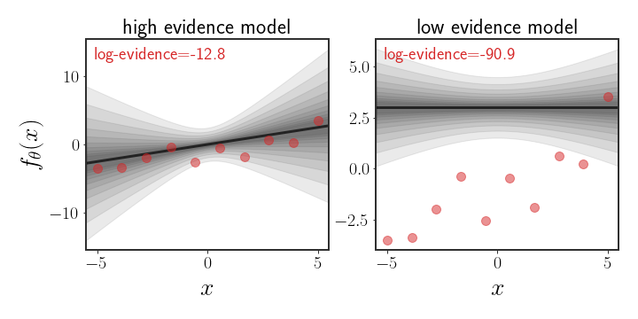
\[\begin{equation} p(\mathcal{D}\mid \Psi)=\intop p(\mathcal{D}\mid \theta) p(\theta\mid \Psi)d\theta =\mathbb{E}_{\theta\mid \Psi}\left[p(\mathcal{D}\mid \theta)\right] \end{equation}\]This is the most direct (and intractable) way to define the evidence, but is a bit more approachable, in an abstract kind of way. Notice that the operation we actually have here is (basically) a sum of all possible likelihoods the data gets under different values of $\theta$ according to the prior (the $p(\mathcal{D}\mid \theta)$ ), weighted by the prior probability. This means that if the data has high likelihood under values of the prior that have high density, then the evidence for the prior will be high. On the other hand, if the area with highest density on the prior isn’t even close to the data, then the evidence will be low. This is shown in the figure below
Choosing Basis Functions
Evidence can be used to decide which basis function to use. At the beginning of this post, I showed an example with two polynomials.
Below, I show the same as figure 2, just for Gaussian basis functions which are defined according to:
\(\begin{equation} h_i(x)=e^{-\frac{\mid \mid x-\mu_i\mid \mid ^2}{2\beta}} \end{equation}\) for some fixed $\beta$ :
The chosen prior for this example is:
\(\begin{equation} \theta\sim\mathcal{N}\left(\left[\matrix{a\\-a}\right],\ I\alpha^2\right) \end{equation}\) for some value of $a$ and $\alpha$ .
Note that while the evidence space looks symmetric, it isn’t exactly so. The evidence for the lower-right corner is slightly higher than that of the upper-right corner. The reason for this is because of the choice of prior, since the defined function is:
\[\begin{equation} f_\theta(x)=\theta_1 h_1(x)+ \theta_2h_2(x)+\eta \end{equation}\]Choosing the Prior Mean
Evidence can also be used to choose which prior is suitable. For instance, suppose that our prior is given by:
\(\begin{equation} \left(\matrix{\theta_0\\ \theta_1}\right)\sim \mathcal{N}\left(\left(\matrix{\mathbb{E}[\theta_0]\\ \mathbb{E}[\theta_1]}\right),\ \ I\alpha^2\right) \end{equation}\) where the function is modeled as $f_\theta(x)=\theta_0 + \theta_1 x+\eta$ . The animation below depicts how the evidence changes when the means $\mathbb{E}[\theta_i]$ are changed:
Maximizing Evidence as Hypothesis Selection
Back in the post about Bayesian decision theory, I introduced which estimators are considered optimal under specific losses and risks. One particular example, actually related to evidence, was that of the 0-1 loss. To jog your memory, in that post we said that if our loss is the same for every wrong example, no matter how far, then the best possible estimator is the MAP estimate. In this sense, if we have to put all our eggs in one basket, the MAP estimator is the way to go.
Choosing the linear regression model and set of basis functions to use is an example of this “putting all our eggs in one basket” scenario. Let’s bunch together the basis functions, prior and noise and call all of these things together a hypothesis. Now suppose we have a set of hypothesis:
\[\begin{equation} \mathcal{H}=\left\{\Psi_i \right\}_{i=1}^{M} \end{equation}\]We now have to choose one of these hypothesis - only one. It’s kind of hard to say “how wrong” a hypothesis is, after all we started this whole debating by saying that the likelihood for a set of points isn’t a good way to choose a model (at the start of the post). Instead, we just want the one that will be closest.
I’m going to assume that all hypothesis are equally as likely, so $p(\Psi_i)=p(\Psi_j)=1/\vert\mathcal{H}\vert$. Then, the MAP estimate under this “hyperprior” over $\mathcal{H}$, given the observed $\mathcal{D}$, is:
\[\begin{equation} \hat{\Psi}=\arg\max_{\Psi\in\mathcal{H}}p\left(\Psi\right)p\left(\mathcal{D}\vert\Psi\right)=\arg\max_{\Psi\in\mathcal{H}}p\left(\mathcal{D}\vert\Psi\right) \end{equation}\]This is exactly the setting we’ve been discussing this whole post.
Regarding Calibration
The evidence is certainly a useful tool for model selection, but it should be used carefully. In particular, relying too much on the evidence without taking care can result in overfitting to the training data. More concisely, high evidence doesn’t equal good generalization! This is because, by design, the marginal likelihood gives high scores to priors which explain the data well.
This is really problematic if we don’t take care to separate the manner in which we choose the prior from the model selection stage. For instance, assume we have some data $\mathcal{D}$ and want to find the model that gives this data the highest possible evidence. Recall that:
\(\begin{equation} p\left(y\mid \Psi\right)=\mathcal{N}\left(y\,\mid \,H\mu_0,\;H\Sigma_0 H^{T}+I\sigma^{2}\right) \end{equation}\) In such a case, we can always define the basis functions/prior such that $H\mu_0=y$ , $\Sigma_0=0$ and $\sigma^2$ is arbitrarily small. This will result in the following, not very helpful, evidence:
\[\begin{equation} p\left(\tilde{y}\mid \Psi\right)=\delta(y) \end{equation}\]which is equal to infinity when $\tilde{y}=y$ , a really good evidence score. However, this is obviously not the model we would want to choose! Such a model will not generalize to any new data, which is basically the definition of overfitting.
While the above is kind of a silly case we won’t see in real life, it still illustrates the problems that may arise when optimizing the evidence. Specifically, if the set of possible models contains many very specific and expressive models, then optimizing on this set of models is prone to overfitting. On the other hand, it could be tempting to iterate over different sets of possible models as we see the results; again, this would just lead to models that are overfit and won’t be calibrated towards new (unseen) data points.
Mitigation
This overfitting problem seems to break the proof we had that choosing according to evidence is optimal, right? However, notice that when we have an infinite number of hypothesis to choose from, all of which we give the same probability, we’ve already infringed on the assumptions we made in the previous section. Where did we go wrong? There is no uniform distribution on a set with an infinite number of members!
Instead, the discussion above is kind of backwards of how we defined the fitting process in the first place; we assumed that we have several priors that (we believe) explain the data equally well, and only then do we want to select one out of these possible priors. In other words, choosing according to evidence should be carried out only if we remain true to the original Bayesian method and choose a set of priors before we ever see the data. Only then should we try to select one of them, so that the selection of the possible set of priors is independent of the data. This, as mentioned, is more in line with the Bayesian philosophy.
Priors all the Way Down
Probably the “true Bayesian method” to overcome these problems is a different approach all together. In the first place, assuming that all these sets of hypotheses we were talking about are equally likely is questionable. Instead, we would want to choose some sort of hyperprior - a prior over the hyperparameters:
\[\psi\sim p(\Psi\mid \xi)\]where $\xi$ are the parameters of the hyperprior.
In such a setting, our posterior distribution will be defined by integrating out the hyperparameters:
\[p(\theta\mid \mathcal{D})=\intop p(\theta\mid \Psi,\mathcal{D})p(\Psi\mid \xi)d\Psi\]This is nice since it bypasses the need to choose a model - simply integrate over all of them, a more Bayesian approach. It also incorporates our beliefs explicitly - in the integral above we explicitly assumed that $\Psi$ is independent of $\mathcal{D}$ !
That said, we have introduced a new complication; how should $\xi$ be chosen? Continuing with this reasoning, shouldn’t we also incorporate a prior over $\xi$, a so called “hyper-hyperprior”, and so on? While these concerns are valid, the “priors all the way down” kind of approach typically stops at a single hyperprior, since it is far enough from the data term. Also, it becomes way too difficult when there’s more than a single hyperprior.
Discussion
Choosing models according to the evidence is a very strong method. In particular, we saw how it can be the optimal method to select which model/prior to use. Actually, showing how to calculate the evidence for linear regression is an extremely useful example - in most cases, calculating the evidence is impossible, but for linear regression there’s a closed form for it!
Something we haven’t fully explored yet is what happens when we have more parameters than data points, something completely illegal in “classical” machine learning but totally fine under the Bayesian paradigm. Starting in the next post, we’re going to use more parameters - sometimes even infinitely many parameters.