The Benefits of Sampling
When the posterior is complex, it is typically quite hard to get a sense for the full distribution. As such, it is common to represent the full distribution using samples from the posterior. In this post we will look at the benefits of doing so.
Throughout most of the previous posts, the focus was Gaussian priors and posteriors. The simplicity of the Gaussian distribution allowed us to directly characterize the full posterior distribution fairly easily - all we needed to describe the whole distribution was the mean (MMSE/MAP) and the covariance of the posterior. In those cases, trying to find the mean or maximum of the posterior makes a lot of sense, as it portrays most of the important aspects of the distribution. However, for more complex distributions, using a single estimate of the parameters (such as the MAP or MMSE) in order to describe the full posterior might not be the best approach.
In this post we will look at an alternative to point estimates (such as the MAP or MMSE), in the form of sampling parameters from the posterior.
The Problem with Point Estimates
First, I’d like to motivate why point estimates might be suboptimal in some cases. We’ll start with an abstract example and then look at more concrete scenarios. Consider the following sketch of a hypothetical posterior distribution:
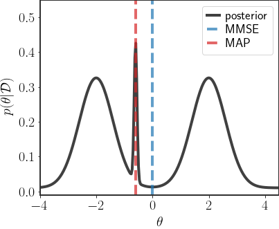
In this, admittedly quite synthetic, scenario both the MAP and MMSE estimates are a rather poor indication of the posterior as a whole. The MMSE falls in a very unlikely region of space, just between both modes. The MAP is better, since it at least has a higher density, but is also located on a rather narrow region of the posterior, which is still a bad description of the overall distribution.
In fact, any single parameter choice on this distribution will misrepresent the distribution as a whole!
What do I mean by that? The distribution has 3 different modes - three separate regions of high probability. If we arbitrarily choose any one of them as the representative for the whole distribution, then we are missing the information about the other 2 modes. Moreover, in cases like this, even choosing the mode according to the MAP estimate describes the least likely mode out of the 3. This is quite different to the Gaussian cases we explored previously, where the mean of the posterior really did give us most of the information we needed about the posterior distribution.
Why Represent the Posterior?
A natural question at this point is: why do we even need estimates that represent the posterior? Don’t we always have access to the full posterior?
This is a valid concern, and if we write down the full posterior (as in the Gaussian cases we considered), we should definitely use all the information we have. But, in many real world cases it is impossible to write down the posterior in closed form, or save the value of the posterior in every place. More concrete examples for this will come in later posts, but let’s consider a simple hypothetical scenario:
Suppose we want to classify images, and are using a neural network with thousands, millions, or billions, of parameters $\theta\in\mathbb{R}^p$ to do so. I’ll write down our classifier as the function $f_\theta(x)$ where $x$ is the image. Recall from the post on discriminative classification that the posterior for a classification problem has no analytical form - we have no formula for the full posterior. Then, to save all information about the posterior would require saving a dense grid of parameter values in a $p$-dimensional space, which is prohibitive beyond 3 dimensions (the number of points on the grid scales exponentially with the dimension). Moreover, calculating the posterior for each parameter choice requires iterating over the whole training set, which can potentially be very large. So each time we want to calculate the value of the posterior, requires a very computationally expensive loop through the whole training set.
Scenarios such as the one above are a good indication of the situation we find ourselves in many real scientific settings. To handle the overwhelming scope of the posterior, we might instead towards representing it with a few point estimates as best as we can.
Multiple Estimates
So, what can we do in such a situation? Instead of describing the full distribution using a single, point estimate, we can save a number of possible parameter choices. Doing so can potentially better represent the full information in the posterior distribution.
One option can be to represent the full posterior distribution using each of the local maxima:
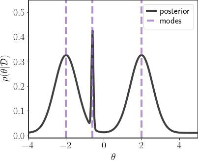
Saving these three points in order to represent the whole distribution makes a lot of sense, especially for GMM posteriors such as these. However, for general distributions it will be quite hard to know how many local maxima there actually are, and finding them will also pose a challenge. Furthermore, there might be situations where the local maxima are still quite bad representatives of the full distribution.
Sampling from the Posterior
A way that (I feel) is more natural to represent the posterior is by leveraging the fact that it is a distribution. Instead of trying to optimize a cost function on the density function, we can instead sample from it directly to get our estimates. These samples then serve as “typical” representatives of what we would expect to observe from the posterior, in the sense that regions of higher mass in the distribution will be more populated than those with lower mass.
In our recurring sketch of a posterior, sampling would give us the following points:
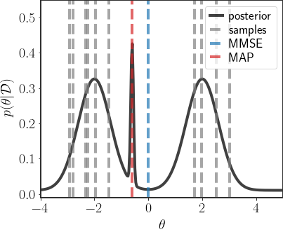
Here I used 10 samples, which are depicted by the positions of the gray, dashed lines. Notice how these samples are more less balanced between the two main modes of the distribution, which really describe most of the density function.
Now, it might seem that sampling is even harder than the optimization needed to find the modes. But in many situations sampling is quite natural and behaves better than optimization. Indeed, the main focus of the following posts will to introduce methods for easily sampling from the posterior in complex scenarios.
Concrete Example: Hierarchical Regression
Hopefully the sketches above gave a clear indication of the problem with point estimates. In this section, I’d like to consider a very real, practical setting where using either the MAP or MMSE makes no sense. To this end, I’d like to explore hierarchical regression.
The setting for hierarchical linear regression is similar to regular linear regression, expect we expect a mixture of different behaviors in the data. We observe data points $\mathcal{D}=\left\{(x_i,y_i)\right\}_{i=1}^N$ which we want to fit using a linear regress, but we assume that each point arose from one out of $K$ different processes, each with their own parameters $\theta_k$ and basis functions $h_k(x)$:
\[y_i=\theta_{k_i}^T h_{k_i}(x_i)+\eta_i\qquad \eta_i\sim\mathcal{N}\left(0,\sigma^2\right)\]For example, we might believe that the $y_i$s are linear or quadratic in $x_i$, and we see a mix of the two behaviors. In this case, the regression problem becomes:
\[y_i=\begin{cases}\theta_1\cdot x_i\\\text{or}\\\theta_2\cdot x_i^2\end{cases}+\eta_i\]Data in such a scenario will look similar to:
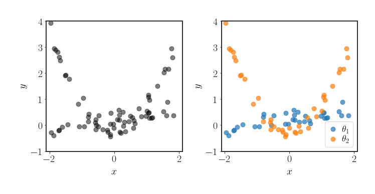
So, to solve this regression problem, we would want to know what the true allocation of each data point is to each of the possible basis functions, and the respective parameters for that basis function. Solving this problem is very nontrivial.
Hierarchical Regression Posterior
Concretely, we have a Gaussian prior over the parameters for every behavior:
\[\theta_k\sim\mathcal{N}\left(\mu_k,\Sigma_k\right)\]with a-priori probability $\pi_k$ for each behavior.
The full posterior is given by:
\[\begin{align} p(\theta\vert \mathcal{D})&=\sum_z p(z,\theta\vert \mathcal{D}) \end{align}\]where $z=\left\{k_i\right\}_{i=1}^N$ is the vector of allocations of each datapoint to the respective behavior. So, while it seems simple in this notation, the above sum actually has $K^N$ different terms - each datapoint can be allocated to each of the different behaviors.
For a given allocation, the term in the summation is:
\[\begin{align} p(\theta\vert \mathcal{D},z) &\propto p(\mathcal{D}\vert \theta,z)\cdot p(\theta\vert z)\\ &= \prod_{i=1}^N\mathcal{N}\left(y_i\vert \ \theta_{k_i}^T h_{k_i}(x_i),\ \sigma^2\right) \cdot \prod_{k=1}^K\mathcal{N}\left(\theta_k\vert \ \ \mu_k,\Sigma_k\right) \end{align}\]This is quite a mess, but for a particular allocation the posterior for each $\theta_k$ can be found simply by considering this as $K$ separate problems.
Samples versus MMSE
In the next post we’ll see how we can sample from the above posterior without explicitly calculating all of it. For now, let’s just look at samples from posterior versus an MMSE estimate:
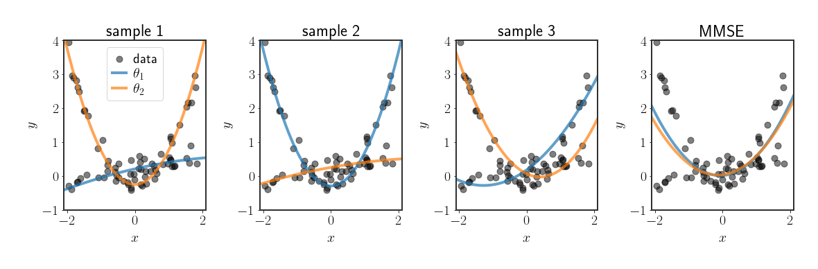
As you can see, in this scenario we see the concrete results of taking the mean over a posterior with multiple modes as the MMSE estimate, which misses most of the data.
This is still quite a simple scenario (and you could “fix” the MMSE in this specific case), but it serves as a very concrete and visual example for the fitting capabilities of sampling from the posterior. Moreover, something we will discuss in the next post is that sampling from this posterior is fairly simple when $K$ is not too large, whereas optimizing the posterior directly would be much more difficult.
Discussion
Hopefully the examples above provide the conceptual basis for why we would want (multiple) samples in order to describe the full posterior distribution, instead of one specific estimate. In the next few posts will be more mathematically involved, and we will delve into how to sample from the posterior. The examples above, while quite simple, will be our motivation to do so.