Gaussian Mixture Models and Expectation Maximization
Gaussian distributions, while simple, are very rigid. In this post we consider Gaussian Mixture Models (GMMs), a more expressive and complex family of distributions.
← Generative classificationBenefits of Sampling →
In all of the posts so far, we pretty much stayed with the Gaussian prior and likelihood, even though many times that might not make much sense. The reason we had to keep everything Gaussian is because anything beyond that complicates the mathematics considerably.
We will now delve a bit more into a class of more expressive priors and noise models. This will illustrate why the math of Bayesian statistics is complicated for many models beyond the Gaussian and will set the stage for some interesting ways to bypass these difficulties.
Gaussian Mixture Models (GMMs)
What is the natural next stage after a Gaussian distribution? A distribution made up of multiple Gaussians!
We’ve already seen this distribution in the previous post for generative classification. Basically, a Gaussian mixture model (GMM) is a convex sum of Gaussians:
\[\begin{align} p(x)=\sum_{k=1}^K\pi_k&\cdot\mathcal{N}\left(x\vert\ \mu_k,\ \Sigma_k\right)\qquad \sum_k\pi_k=1\qquad \pi_k\ge0\\ \Leftrightarrow x&\sim \text{GMM}\left(\\{\pi_k,\mu_k,\Sigma_k\\}_{k=1}^K\right) \end{align}\]The values $\pi_k$ are sometimes called the mixture probabilities, as they dictate the probability to end up in one of the Gaussians, which are also called centers or clusters.
In 1D, these distributions look like a sum of all of the Gaussians:
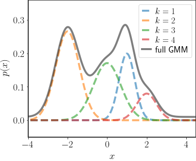
As you can see in the example above, the GMM distribution captures very complex behaviors. In fact, if you have enough Gaussians, GMMs can capture most continuous distributions on all of $\mathbb{R}$. Below you can find an interactive version of the above plot:
We can also write the joint probability of $x$ and a single cluster:
\[p\left(x,k\right)=p\left(x\vert k\right)p\left(k\right)=\pi_{k}\cdot\mathcal{N}\left(x\vert\ \mu_k,\Sigma_k\right)\]The conditional distributions will also help us in the near future, so let’s write them down:
\[\begin{align} p\left(x\vert k\right)&=\mathcal{N}\left(x\vert\ \mu_k,\Sigma_k\right) \\ p\left(k\vert x\right)&=\frac{p\left(k\right)p\left(x\vert k\right)}{p\left(x\right)}=\frac{\pi_{k}\cdot\mathcal{N}\left(x\vert\ \mu_k,\Sigma_k\right)}{\sum_{k'}\pi_{k'}\cdot \mathcal{N}\left(x\vert\ \mu_{k'},\Sigma_{k'}\right)} \end{align}\]and we have our full set of equations.
Sampling from a GMM is also pretty straightforward once we know how to sample from a Gaussian. The only change is that we use 2 steps instead of one. Our first step is to sample:
\[k\sim p\left(k\right)\]which just means sampling $k$ proportional to the assignment probabilities, $\pi_{k}$. After we have chosen $k$, we simply sample a new point $x$ from the $k$-th Gaussian using the conditional distribution:
\[x\vert k\sim\mathcal{N}\left(\mu_{k}, \Sigma_{k}\right)\]GMM Log-Likelihood
We typically want to be able to fit a GMM to a given data set $\mathcal{D}=\left\{ x_{i}\right\}_{i=1}^{N}$ in order to learn a GMM prior, and not assume that we already know all of the parameters ahead of time. That is, we want to find the $\pi_{k}$s, the $\mu_{k}$s and the $\Sigma_{k}$s that describe the sample distribution as best as we can. To do this we can use MLE, in which case we need to know what the log-likelihood of the data set is according to a given model. The log-likelihood is given by:
\[\log p\left(\mathcal{D}\vert \theta\right)=\sum_{i=1}^{N}\log\left[\sum_{k}\pi_{k}\cdot\mathcal{N}\left(x_i\vert\ \mu_k,\Sigma_k\right)\right]\]… and we’re in deep trouble. Since we don’t know to which of the Gaussians each sample $x_{i}$ actually belongs, we don’t know how to separate the term in the logarithm into something that’s easy to work with. This is a problem; we don’t know how to easily find the maximum according to this and it is now clearly not convex.
How is this different from GDA?
The above log-likelihood is very similar to a version we have already seen in the previous post, with a slight modification. Suppose that, instead, our data set was composed of the pairs $\mathcal{D}=\left\{ x_{i},y_{i}\right\}_{i=1}^{N}$ where $y_{i}$ is the classification of each point, as in GDA. In this case, the log-likelihood becomes (as we have already seen):
\[\log p\left(\mathcal{D}\vert\theta\right)=\sum_{i=1}^{N}\sum_{k}\mathbb{I}\left[y_{i}=k\right]\left[\log\pi_{k}+\log\mathcal{N}\left(x_{i}\vert\ \mu_{k}, \Sigma_{k}\right)\right]\]which we can easily optimize. This is because we know which Gaussian is responsible for each of the data points, so we can estimate the mean and covariance for the set of points for each one of the Gaussians.
However, when our data set is comprised of $\left\{ x_{i}\right\}_{i=1}^{N}$, the $y_{i}$s are hidden from us and we can’t directly rely on them when maximizing the log-likelihood. That is, we can’t know ahead of time which Gaussian is responsible for each one of the data points. In such a scenario, how can we “separate” the different Gaussians from each other?
Using a GMM Prior for Bayesian Linear Regression
Suppose we have:
\[\theta\sim\text{GMM}\left(\pi,\left\{ \mu_{k}\right\}_{k=1}^{K},\left\{ \Sigma_{k}\right\}_{k=1}^{K}\right)\]and we want to solve the regular Bayesian linear regression problem:
\[y=h^{T}\left(x\right)\theta+\eta\qquad\eta\sim\mathcal{N}\left(0,I\sigma^{2}\right)\]Then the posterior distribution will also be a GMM, with the same number of centers as the prior:
\[\begin{align} p(\theta|\mathcal{D})&=\frac{1}{p(\mathcal{D})}p(\mathcal{D},\theta)\\ &= \frac{1}{p(\mathcal{D})}\sum_kp(\mathcal{D},\theta,k)\\ &= \sum_k\frac{\pi_k\cdot(\mathcal{D}\vert k)}{p(\mathcal{D})}\cdot p (\theta\vert\mathcal{D},k) \end{align}\]This is essentially like finding the posterior for $K$ different linear regressors, each with their own prior, and bringing them together into a GMM where the mixture coefficients are decided according to their evidences.
Note that once again, if we want to find the MAP estimator, we fall into the same problem we had when trying to find the ML estimate for a GMM. In both of these cases we are trying to maximize a function that isn’t convex. However, had we known the “real” Gaussian responsible for each data point, we would be able to solve this problem quite easily.
MMSE under a GMM prior
The MMSE, on the other hand, is quite easy to calculate for a GMM prior:
\[\begin{align} \hat{\theta}_{\text{MMSE}}&=\sum_{k=1}^{K}q_{k}\hat{\mu}_{k}\\ &=\frac{\sum_{k=1}^{K}p\left(\mathcal{D}\vert k\right)\left(\Sigma_{k}^{-1}+\frac{1}{\sigma^{2}}H^{T}H\right)^{-1}\left(H^{T}\frac{1}{\sigma^{2}}y+\Sigma_{k}^{-1}\mu_{k}\right)}{\sum_{k'}p\left(\mathcal{D}\vert k'\right)} \end{align}\]However, the MMSE solution is in general less favorable for a GMM posterior, since if all of the centers in the GMM are very different from each other, then the MMSE result can have a very low density:
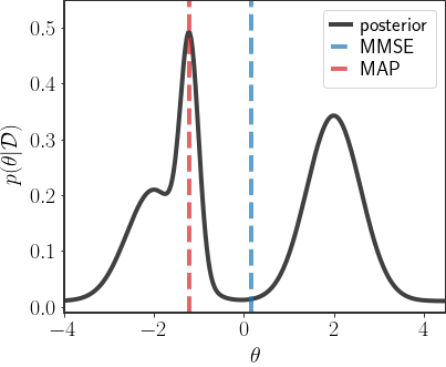
So many times we may not want to use the MMSE estimator, since we may want something that gives us a better indication of the general behavior of the data.
Using the MAP estimate is a bit better, since we at least use something with a higher density, but it could fall on a mode that is very narrow, as in the example above. In this case, because the region in space is so narrow, actually sampling a point in that region is relatively unlikely. So, sometimes the MAP estimate might not be typical.
Difficulties with Complex Distributions
Before explaining how we might go above solving both of the problems above, let’s try to understand what we’re up against again.
The GMM describes a distribution much more complex than a single Gaussian. Unlike a single Gaussian, the density of the GMM can potentially have many maxima and minima. In the past, for the Gaussian distribution, we looked at either the MLE solution or the MAP estimate - both of which are the maximum of a density function, the first the maximum of the likelihood and the second the posterior. However, because GMMs have multiple peaks, there are multiple local maximas. How then, can we optimize these complex distributions?
One option is to just try to differentiate and equate the likelihood/posterior to zero, as we did before. But, if you try to do this you’ll quickly find that you’re in deep trouble. Because the log-likelihood, unlike the Gaussian distribution, is not convex, doing so is usually intractable. That is, an analytical solution is hard, if not impossible, to find.
Naturally, this problem is not unique to GMMs. If we want to use complex distributions, either as likelihoods or as priors, we have to find new manners of optimizations. A relatively simple method is to just use gradient ascent on the density in order to find a local maximum. Below we explore an alternative solution which can be a bit faster, and works particularly well for GMMs.
Expectation Maximization Algorithm
The Expectation-Maximization (EM) algorithm allows us to solve both problems of MLE estimation for the GMM parameters, as well as MAP estimation under a GMM prior in linear regression. However, the EM algorithm applies for even more diverse scenarios, and in particular in settings where some information is missing which would otherwise render the problem as quite easy to solve. In the most intuitive sense, the EM tries to “fill in” the missing information using the model itself, and then updates the model using the estimated values for the missing information. For the GMM cases above, the EM algorithm basically iterates between classifying the data points to each Gaussian, and then updating the parameters of the Gaussians using this classification - which is repeated iteratively.
Formally, the EM algorithm is defined as:
EM Algorithm: Suppose we want to find the value of $\theta$ that maximizes some density $p\left(x\vert\theta\right)$. In addition, suppose that given another variable $z$ - which we do not observe - the log-density $\log p\left(x,z\vert\theta\right)$ is easy to maximize. The expectation maximization (EM) algorithm alternates between the following two steps:
\[\begin{align} \text{E-step:}&\quad Q\left(\theta\vert\theta_{t-1}\right)\stackrel{\Delta}{=}\mathbb{E}_{z\vert x,\theta_{t-1}}\left[\log p\left(x,z\vert\theta\right)\right]\\ \text{M-step:}&\quad \theta_{t}\stackrel{\Delta}{=}\arg\max_{\theta}Q\left(\theta\vert\theta_{t-1}\right) \end{align}\]where $t$ is the iteration of the algorithm. The algorithm itself repeats the E and M-steps iteratively until convergence is reached and returns an $\theta_T$ which approximately maximizes the probability $p\left(x\vert\theta\right)$.
The reverse is also possible. If we want to maximize $p\left(\theta\vert x\right)$, an equivalent algorithm with the following E-step can be used:
\[\text{E-step:}\quad Q\left(\theta\vert\theta_{t-1}\right)\stackrel{\Delta}{=}\mathbb{E}_{z\vert x,\theta_{t-1}}\left[\log p\left(\theta,z\vert x\right)\right]\]
Notice that the algorithm is explicitly designed to solve maximization problems when we have some missing information, which we called $z$ in the above explanation of the EM algorithm. Essentially, the E-step estimates the missing values of $z$ using the MMSE under the previous version of the model. Once we have an estimation of the values which are missing, maximization becomes simpler (if $\log p(x,z\vert\theta)$ is easy to optimize).
The above definition is the most general definition for the EM algorithm. If we try to maximize $p\left(\mathcal{D}\vert\theta\right)$ then this will be an (approximate) MLE algorithm. On the other hand, if we want to maximize $p\left(\theta\vert\mathcal{D}\right)$, then the algorithm will be a MAP algorithm (approximately). In both cases, if we have a GMM and assume that the values of the $k$s are known, then the log-probabilities $p\left(\mathcal{D},k\vert\theta\right)$ and $p\left(\theta,k\vert \mathcal{D}\right)$ are easy to maximize, which lands us right in the area where the EM algorithm is the most useful.
Proof of correctness for the EM algorithm
Theorem: at each iteration $t$ of the EM algorithm:
\[p\left(x\vert\theta_{t}\right)\ge p\left(x\vert\theta_{t-1}\right)\]That is, the EM algorithm can only increase the density $p\left(x\vert\theta\right)$.
Proof: To prove the above theorem, let’s define a new function:
\[\tilde{Q}\left(\theta\vert \theta_{t-1}\right) \stackrel{\Delta}{=} Q\left(\theta\vert \theta_{t-1}\right)-\sum_{z}p\left(z\vert x,\theta_{t-1}\right)\log p\left(z\vert x,\theta_{t-1}\right)\]Notice that if we find the $\theta$ that maximizes $\tilde{Q}\left(\theta\vert \theta_{t-1}\right)$, then it will be the same $\theta$ that maximizes $Q\left(\theta\vert \theta_{t-1}\right)$, since the added term is constant with respect to \theta. If we open up this expression completely, we will see that:
\[\begin{align} \tilde{Q}\left(\theta\vert\theta_{t-1}\right) &=\sum_{z}p\left(z\vert x,\theta_{t-1}\right)\log p\left(x,z\vert\theta\right)-\sum_{z}p\left(z\vert x,\theta_{t-1}\right)\log p\left(z\vert x,\theta_{t-1}\right)\\ &=\sum_{z}p\left(z\vert x,\theta_{t-1}\right)\left[\log p\left(z\vert x,\theta\right)+\log p\left(x\vert\theta\right)\right]-\sum_{z}p\left(z\vert x,\theta_{t-1}\right)\log p\left(z\vert x,\theta_{t-1}\right)\\ &=\sum_{z}p\left(z\vert x,\theta_{t-1}\right)\log p\left(x\vert\theta\right)+\sum_{z}p\left(z\vert x,\theta_{t-1}\right)\log\frac{p\left(z\vert x,\theta\right)}{p\left(z\vert x,\theta_{t-1}\right)}\\ &=\log p\left(x\vert\theta\right)-\text{KL}\left(p\left(z\vert x,\theta_{t-1}\right)\,\vert\vert\,p\left(z\vert x,\theta\right)\right) \end{align}\]where $\text{KL}\left(\cdot\,\vert\vert\,\cdot\right)$ is the Kullback-Leibler (KL) divergence. The KL divergence is a popular way to measure the distance between distributions and has a few neat properties. Even though it doesn’t look like it, for any two distributions $S$ and $L$, the KL divergence is non-negative:
\[\text{KL}\left(S\,\vert \vert \,L\right)\ge0\]where equivalence is reached if and only if $S=L$. In this case, this means that:
\[\begin{align} \forall\theta\quad\log p\left(x\vert \theta\right) &\ge\tilde{Q}\left(\theta\vert \theta_{t-1}\right)\\ \log p\left(x\vert \theta_{t-1}\right) &=\tilde{Q}\left(\theta_{t-1}\vert \theta_{t-1}\right) \end{align}\]Additionally, recall that we defined the M-step as:
\[\theta_{t}=\arg\max_{\theta}Q\left(\theta\vert \theta_{t-1}\right)=\arg\max_{\theta}\tilde{Q}\left(\theta\vert \theta_{t-1}\right)\]in which case we can always say that:
\[\begin{align} \log p\left(x\vert \theta_{t}\right)&=\tilde{Q}\left(\theta_{t}\vert \theta_{t}\right)\ge\tilde{Q}\left(\theta_{t}\vert \theta_{t-1}\right)\\ &=\max_{\theta}\tilde{Q}\left(\theta\vert \theta_{t-1}\right) \ge\tilde{Q}\left(\theta_{t-1}\vert \theta_{t-1}\right)\\ &=\log p\left(x\vert \theta_{t-1}\right)\\ \Leftrightarrow p\left(x\vert \theta_{t}\right) &\ge p\left(x\vert \theta_{t-1}\right) \end{align}\]$\square$
Some Things to Look Out For
• EM isn’t guaranteed to converge to the global maximum of $p\left(x\vert \theta\right)$! The only guarantee of the EM algorithm is that in each iteration the log-likelihood can only increase or stay the same i.e. that: $p\left(x\vert \theta_{t}\right)\ge p\left(x\vert \theta_{t-1}\right)$.
• In addition, notice that the whole process is dependent on the initial conditions $\theta_{0}$. This means that we may arrive at very different solutions for different initialization of the parameters. Since the EM algorithm is only guaranteed to converge to a local maximum, this means that it may be a good idea to use several initialization and then choose the one that has the best performance after convergence. Another option is to devise a scheme where there are some guarantees on the solutions the EM algorithm will converge to.
• Note that it isn’t necessary to find the maximum at each step, only to improve the score function $Q\left(\theta\vert \theta_{t-1}\right)$ at each iteration, for our proof to still be valid.
EM for Estimation of GMM Parameters
To apply the EM algorithm to GMMs, we need to explicitly define the E-step and the M-step. In GMMs, the hidden variables are the association of each point to each Gaussian, where each point $x_{i}$ has an association with a Gaussian, which we will call $y_{i}$. So our hidden variables are the set $y=\left\{ y_{i}\right\}_{i=1}^{N}$. The observed variables are, of course, the $x_{i}$s.
E-Step
In previous sections we already defined the joint likelihood, so all that remains is to find the conditional expectation:
\[\begin{align} Q\left(\theta\vert \theta_{t}\right)&=\mathbb{E}_{y\vert x,\theta_{t}}\left[\log p\left(x,y\vert \theta\right)\right] \\ &=\mathbb{E}_{y\vert x,\theta_{t}}\left[\sum_{i=1}^{N}\sum_{k}\mathbb{I}\left[y_{i}=k\right]\left(\log\pi_{k}+\log \mathcal{N}\left(x_i\vert \mu_k,\Sigma_k\right)\right)\right]\\ &=\sum_{i=1}^{N}\sum_{k}\mathbb{E}_{y_{i}\vert x_{i},\theta_{t}}\left[\mathbb{I}\left[y_{i}=k\right]\left(\log\pi_{k}+\log\mathcal{N}\left(x_i\vert \mu_k,\Sigma_k\right)\right)\right]\\ &=\sum_{i=1}^{N}\sum_{k}\mathbb{E}_{y_{i}\vert x_{i},\theta_{t}}\left[\mathbb{I}\left[y_{i}=k\right]\right]\left(\log\pi_{k}+\log\mathcal{N}\left(x_i\vert \mu_k,\Sigma_k\right)\right) \end{align}\]Let’s separate the expectation from the rest of the equation for brevity. In this case we have:
\(\begin{align} \mathbb{E}_{y_{i}\vert x_{i},\theta_{t}}\left[\mathbb{I}\left[y_{i}=k\right]\right] &=\sum_{k'}\mathbb{I}\left[y_{i}=k\right]p\left(y_{i}=k'\vert x_{i},\theta_{t}\right)\\ &=p\left(y_{i}=k\vert x_{i},\theta_{t}\right)\\ &=\frac{\pi_{k}^{\left(t\right)}\mathcal{N}\left(x_{i}\vert\ \mu_{k}^{\left(t\right)}\Sigma_{k}^{\left(t\right)}\right) }{\sum_{k'}\pi_{k'}^{\left(t\right)}\mathcal{N}\left(x_{i}\vert\mu_{k'}^{\left(t\right)}, \Sigma_{k'}^{\left(t\right)}\right)} \end{align}\) where $\pi_{k}^{\left(t\right)}$, $\mu_{k}^{\left(t\right)}$ and $\Sigma_{k}^{\left(t\right)}$ are the parameters in the $t$-th iteration. These variables are called the responsibilities and they describe the probability that the $i$-th sample originates from the $k$-th cluster. We will define the following variable for the responsibilities for simplicity:
\[r_{ik}^{\left(t\right)}\stackrel{\Delta}{=}\frac{\pi_{k}^{\left(t\right)}\mathcal{N}\left(x_{i}\vert\ \mu_{k}^{\left(t\right)}\Sigma_{k}^{\left(t\right)}\right) }{\sum_{k'}\pi_{k'}^{\left(t\right)}\mathcal{N}\left(x_{i}\vert\mu_{k'}^{\left(t\right)}, \Sigma_{k'}^{\left(t\right)}\right)}\]and we will usually just write $r_{ik}$ (without the superscript with the iteration number) instead, since the iteration can be understood from context.
Plugging the responsibilities back into the log-likelihood we get the full E-step:
\[Q\left(\theta\vert \theta_{t}\right)=\sum_{i=1}^{N}\sum_{k}r_{ik}\left(\log\pi_{k}+\log\mathcal{N}\left(x_i\vert\mu_k,\Sigma_k\right)\right)\]Note that this involves explicitly calculating the $N\times k$ different values for the responsibilities.
M-Step
We now have to differentiate $Q\left(\theta\vert \theta_{t}\right)$ by each of the parameters in order to find their maximum.
Finding $\pi_{k}$ - to find $\pi_{k}$, we have to define the Lagrangian and differentiate it with respect to $\pi_{k}$:
\(\begin{align} \frac{\partial}{\partial\pi_{k}}\mathcal{L} &=\frac{\partial}{\partial\pi_{k}}\left(Q\left(\theta\vert \theta_{t}\right)-\lambda\left(\sum_{k}\pi_{k}-1\right)\right)\\ &=\sum_{i=1}^{N}r_{ik}\frac{1}{\pi_{k}}-\lambda\stackrel{!}{=}0\\ \Rightarrow \pi_{k}&=\frac{\sum_{i=1}^{N}r_{ik}}{\lambda} \end{align}\)
Using the condition on $\pi_{k}$ we have: \(\begin{align} \sum_{k}\pi_{k} &=\sum_{k}\frac{\sum_{i=1}^{N}r_{ik}}{\lambda}\\&=\frac{1}{\lambda}\sum_{k}\sum_{i}r_{ik}\\ &=\frac{1}{\lambda}N\stackrel{!}{=}1\\&\Rightarrow\lambda=N \end{align}\) and we get: $\hat{\pi}_{k}^{ML}=\frac{1}{N}\sum_{i=1}^{N}r_{ik}$
Finding $\mu_{k}$ - notice that deriving by $\mu_{k}$ we get almost the same expression as for a single Gaussian, only each sample is reweighed by $r_{ik}$: \(\begin{align} \frac{\partial}{\partial\mu_{k}}Q\left(\theta\vert \theta_{t}\right)& =\sum_{i}r_{ik}\frac{\partial}{\partial\mu_{k}}\left(-\frac{1}{2}\left(x_{i}-\mu_{k}\right)^{T}\Sigma_{k}^{-1}\left(x_{i}-\mu_{k}\right)\right)\\ &=-\sum_{i}r_{ik}\Sigma_{k}^{-1}\left(x_{i}-\mu_{k}\right)\stackrel{!}{=}0\\ &\Rightarrow \sum_{i}r_{ik}\mu_{k}=\sum_{i}r_{ik}x_{i}\\ &\Rightarrow \hat{\mu}_{k}^{ML}=\frac{\sum_{i}r_{ik}x_{i}}{\sum_{i}r_{ik}} \end{align}\)
Finding $\Sigma_{k}$ - the covariance can also be found when considering it as a weighted variant of the single Gaussian: \(\hat{\Sigma}_{k}^{ML}=\frac{\sum_{i}r_{ik}\left(x_{i}-\hat{\mu}_{k}^{ML}\right)\left(x_{i}-\hat{\mu}_{k}^{ML}\right)^{T}}{\sum_{i}r_{ik}}\)
Full Update Steps
The full algorithm is given by iterating:
\[\begin{align} r_{ik} &\stackrel{\Delta}{=}\frac{\pi_{k}^{\left(t-1\right)}\mathcal{N}\left({x_{i}}\vert{\mu_{k}^{\left(t-1\right)}},{\Sigma_{k}^{\left(t-1\right)}}\right)}{\sum_{k'}\pi_{k'}^{\left(t-1\right)}\mathcal{N}\left({x_{i}}\vert{\mu_{k'}^{\left(t-1\right)}},{\Sigma_{k'}^{\left(t-1\right)}}\right)}\\ \pi_{k}^{\left(t\right)} &=\frac{1}{N}\sum_{i=1}^{N}r_{ik}\\ \mu_{k}^{\left(t\right)} &=\frac{\sum_{i}r_{ik}x_{i}}{\sum_{i}r_{ik}}\\ \Sigma_{k}^{\left(t\right)} &=\frac{\sum_{i}r_{ik}\left(x_{i}-\mu_{k}^{\left(t\right)}\right)\left(x_{i}-\mu_{k}^{\left(t\right)}\right)^{T}}{\sum_{i}r_{ik}} \end{align}\]Examples
In low dimensions, the EM algorithm for ML estimation of the GMM parameters is quite easy to implement, and very efficient. It also serves for some really cool visualizations:
What are we seeing here? Well, the points are the observed data points, to which we want to fit a GMM. At each iteration of the EM algorithm, the E-step assigns the probabilities of each Gaussian to each point, so here I colored the points according to the Gaussian which has the highest responsibility. The solid ellipses are the Gaussians at each step. The Gaussians are randomly initialized, and fairly quickly converge to the correct distribution (the dashed, gray ellipses).
We can now go crazy and consider more complex distributions of points:
EM for Linear Regression with GMM Priors
When using a GMM prior under a linear regression problem, we want to maximize:
\[p\left(\theta\vert \mathcal{D}\right)=\sum_{k=1}^{K}q_{k}\cdot\mathcal{N}\left(\theta\,\vert \,\hat{\mu}_{k},\hat{\Sigma}_{k}\right)\]where:
\[\begin{align} q_k &= \frac{\pi_k\cdot p(\mathcal{D}\vert k)}{\sum_{k'}\pi_{k'}\cdot p(\mathcal{D}\vert k')}\\ \hat{\Sigma}_k &= \left(\Sigma_k^{-1}+\frac{1}{\sigma^2}H^TH\right)^{-1}\\ \hat{\mu}_k &=\hat{\Sigma}_k\left(\Sigma_k^{-1}\mu_k+\frac{1}{\sigma^2}H^Ty\right) \end{align}\]As stated before, this is difficult to maximize. Our hidden variable is $k$ (similar to before) where $p\left(\theta,k\vert \mathcal{D}\right)$ is easy to maximize.
E-Step
Let’s find the $Q\left(\cdot\,\vert \,\cdot\right)$, which will define the EM algorithm for finding the MAP solution. We want to find:
\[Q\left(\theta\vert \theta_{t-1}\right)\stackrel{\Delta}{=}\sum_{k}p\left(k\vert \mathcal{D},\theta_{t-1}\right)\log p\left(\theta,k\vert \mathcal{D}\right)\]Notice that:
\[\begin{align} p\left(k\vert \mathcal{D},\theta\right) &=\frac{p\left(k\vert \mathcal{D}\right)p\left(\theta\vert k,\mathcal{D}\right)}{\sum_{k'}p\left(k'\vert \mathcal{D}\right)p\left(\theta\vert k',\mathcal{D}\right)}\\ &=\frac{q_{k}\mathcal{N}\left(\theta\,\vert \,\hat{\mu}_{k},\,\hat{\Sigma}_{k}\right)}{\sum_{k'}q_{k'}\mathcal{N}\left(\theta\,\vert \,\hat{\mu}_{k'},\,\hat{\Sigma}_{k'}\right)}\\ &\stackrel{\Delta}{=}\hat{r}_{k}\left(\theta\right) \end{align}\]where the $\hat{r}_{k}\left(\cdot\right)$s are the responsibilities of each Gaussian as we defined before, only under the posterior distribution. We can now write the update function needed in the E-step:
\[\begin{align} Q\left(\theta\vert \theta_{t-1}\right) &=\sum_{k}\hat{r}_{k}\left(\theta_{t-1}\right)\left[\log p\left(k\vert \mathcal{D}\right)+\log p\left(\theta\vert k,\mathcal{D}\right)\right]\\ &=\sum_{k}\hat{r}_{k}\left(\theta_{t-1}\right)\left[\log q_{k}+\log\mathcal{N}\left(\theta\,\vert \,\hat{\mu}_{k},\,\hat{\Sigma}_{k}\right)\right] \end{align}\]M-Step
Of course, we will want to find the $\theta$ that maximizes the above equation in the M-Step. This will be equivalent to finding:
\[\begin{align} \theta_{t} &=\arg\max_{\theta}Q\left(\theta\vert \theta_{t-1}\right)\\ &=\arg\max_{\theta}\sum_{k}\hat{r}_{k}\left(\theta_{t-1}\right)\left[\log q_{k}+\log\mathcal{N}\left(\theta\,\vert \,\hat{\mu}_{k},\,\hat{\Sigma}_{k}\right)\right]\\ &=\arg\max_{\theta}\sum_{k}\hat{r}_{k}\left(\theta_{t-1}\right)\log\mathcal{N}\left(\theta\,\vert \,\hat{\mu}_{k},\,\hat{\Sigma}_{k}\right)\\ &=\arg\min_{\theta}\frac{1}{2}\sum_{k}\hat{r}_{k}\left(\theta_{t-1}\right)\left(\theta-\hat{\mu}_{k}\right)^{T}\hat{\Sigma}_{k}^{-1}\left(\theta-\hat{\mu}_{k}\right)\\ &=\arg\min_{\theta}J\left(\theta\right) \end{align}\]The function $J\left(\cdot\right)$ is a sum of quadratic functions, so to find the minimum we can simply differentiate and equate to 0:
\[\begin{align} \frac{\partial J\left(\theta\right)}{\partial\theta} &=\frac{1}{2}\sum_{k}\hat{r}_{k}\left(\theta_{t-1}\right)\frac{\partial}{\partial\theta}\left(\theta-\hat{\mu}_{k}\right)^{T}\hat{\Sigma}_{k}^{-1}\left(\theta-\hat{\mu}_{k}\right)\\ &=\sum_{k}\hat{r}_{k}\left(\theta_{t-1}\right)\hat{\Sigma}_{k}^{-1}\left(\theta-\hat{\mu}_{k}\right)\stackrel{!}{=}0\\ \Leftrightarrow &\left(\sum_{k}\hat{r}_{k}\left(\theta_{t-1}\right)\hat{\Sigma}_{k}^{-1}\right)\theta=\sum_{k}\hat{r}_{k}\left(\theta_{t-1}\right)\hat{\Sigma}_{k}^{-1}\hat{\mu}_{k}\\ \Leftrightarrow \theta_{t}&=\left[\sum_{k}\hat{r}_{k}\left(\theta_{t-1}\right)\hat{\Sigma}_{k}^{-1}\right]^{-1}\left[\sum_{k}\hat{r}_{k}\left(\theta_{t-1}\right)\hat{\Sigma}_{k}^{-1}\hat{\mu}_{k}\right] \end{align}\]Full Update Steps
So the full algorithm is given by iterating:
\[\begin{align} \hat{r}_{k} &\stackrel{\Delta}{=}\frac{q_{k}\mathcal{N}\left(\theta_{t-1}\,\vert \,\hat{\mu}_{k},\,\hat{\Sigma}_{k}\right)}{\sum_{k'}q_{k'}\mathcal{N}\left(\theta_{t-1}\,\vert \,\hat{\mu}_{k'},\,\hat{\Sigma}_{k'}\right)} \theta_{t} \\&=\left[\sum_{k}\hat{r}_{k}\hat{\Sigma}_{k}^{-1}\right]^{-1}\left[\sum_{k}\hat{r}_{k}\hat{\Sigma}_{k}^{-1}\hat{\mu}_{k}\right] \end{align}\]In fact, we can (slightly) simplify this by noticing that:
\[\hat{r}_{k}=\frac{1}{Z}q_{k}\mathcal{N}\left(\theta_{t-1}\,\vert \,\hat{\mu}_{k},\,\hat{\Sigma}_{k}\right)\stackrel{\Delta}{=}\frac{1}{Z}r_{k}\]Plugging this into the M-step:
\[\begin{align} \theta_{t} &=\left[\frac{1}{Z}\sum_{k}r_{k}\hat{\Sigma}_{k}^{-1}\right]^{-1}\left[\frac{1}{Z}\sum_{k}r_{k}\hat{\Sigma}_{k}^{-1}\hat{\mu}_{k}\right]\\ &=\left[\sum_{k}r_{k}\hat{\Sigma}_{k}^{-1}\right]^{-1}\left[\sum_{k}r_{k}\hat{\Sigma}_{k}^{-1}\hat{\mu}_{k}\right]\\ &=\left[\sum_{k}p\left(k,\theta_{t-1}\vert \mathcal{D}\right)\hat{\Sigma}_{k}^{-1}\right]^{-1}\left[\sum_{k}p\left(k,\theta_{t-1}\vert \mathcal{D}\right)\hat{\Sigma}_{k}^{-1}\hat{\mu}_{k}\right] \end{align}\]Discussion
Even though the definition of the GMM is pretty simple, it already allows us to define much more expressive distributions than the single Gaussian. At the same time, the added expressivity introduces new complexities which we might not have considered before. That being said, GMMs are still rather interpretable, which makes them perfect subjects for the consideration of these new complexities.
I briefly touched on why finding the average under a GMM posterior might be considered sub-optimal. Instead, we saw how to optimize a GMM likelihood or posterior. However, when the distribution has multiple modes this might not be the best strategy, either. In the next post we will see why and start considering alternatives.